Curse of dimensionality
Table of contents
1. Basic concept
All the machine learning models suffer from the same fundamental problem. Suppose a dataset has a huge number of features as compared to the number of datapoints. In that case, a sufficiently complex algorithm will more easily overfit. The model will generalize poorly- this is because the model can quickly memorize the data since more features are used to differentiate the datapoints. Instead, if we have a small number of features for the same amount of data, it is harder for the model to learn the relevant features, and it will most certainly underfit.
So what is the right amount of data versus the number of features? A simple criterion can be the following. Suppose we have a binary classification problem with a single feature $x$ that can take $n$ distinct values. Suppose $m$, the number of datapoints is vast. In that case, we have enough datapoints to calculate the empirical probabilities $P(c|x)$ with relative confidence, where $c=0,1$ is the class (we can use histograms for that purpose). We can use the set of empirical probabilities as a classifier- the predictor is the class with a higher probability. On the other hand, if $m$ is smaller than $n$ then the data is too sparse, and we cannot rely on the empirical probabilities. Similarly, if we have an additional feature that can also take $n$ distinct values, we need $m$ to be larger than $n^2$. In general, if the feature space is $d$-dimensional, we need $m\gg n^d$. The same applies to continuous features. One can assume that $n=2^{64}$ for a 64-bit computer, and still the necessary data grows exponentially with the number of dimensions.
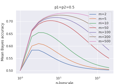
A more detailed analysis, as explained in the following section, shows an optimal $n_{opt}$ for which the accuracy is the best possible. For $n>n_{opt}$ the model prediction deteriorates until it starts performing as an empirical model given by the classes’ relative frequencies. That is, when the number of features is large, the data becomes so sparse that the best we can do is to draw the labels according to their probabilities $P(c=0,1)$.
2. Hughes phenomenon
Suppose we have a binary classification problem with classes $c_1,c_2$ and a training set of $m$ samples with a feature $x$ that can take $n$ values $x_i$. Intuitively having a very large dataset with only very few features, that is, $n\ll m$ may lead to difficulties in learning because there may not be enough information to correctly classify the samples. On the other hand, a small dataset as compared to a very large number of features, $n\gg m$, means that we need a very complex hypothesis function which may lead to overfitting. So what is the optimal number $n_{opt}$?
We use the Bayes optimal classifier. In this case we choose the class that has higher probability according to the rule
\[\tilde{c}_i=\text{argmax}_{j=1,2}P(c_j|x)\]where $\tilde{c}_i$ is the predicted class and $P(c,x)$ is the true distribution. The accuracy of the Bayes optimal classifier is then
\[\sum_{x,c}\mathbb{1}_{c,\tilde{c}}P(c,x)=\sum_{x,\tilde{c}=\text{argmax P(c|x)}} P(\tilde{c},x)=\sum_x[\text{max}_c P(c|x)] P(x) =\sum_x [\text{max}_c P(x|c)P(c)]\]Lets define $p_{c_1}\equiv P(c_1)$ and $p_{c_2}\equiv P(c_2)$. The Bayes accuracy can be written as
\[\sum_{x=x_1}^{x_n} \text{max}\left(P(x|c_1)p_{c_1},P(x|c_2)p_{c_2}\right)\]We ought to study the Bayes accuracy over all possible environment probabilities $P(x|c_1)$ and $P(x|c_2)$.
Statistical approach
To do this we define
\[\begin{equation*}\begin{split}u_i&\equiv P(x_i|c_1), i=1\ldots n\\ v_i&\equiv P(x_i|c_2), i=1\ldots n\end{split}\end{equation*}\]and assume that $u,v$ are themselves random variables. The measure for $u_i,v_i$ can be calculated from the expression
\[dP(u_1,u_2,\ldots,u_n,v_1,v_2,\ldots,v_n)=Ndu_1du_2\ldots du_{n-1}dv_1dv_2\ldots dv_{n-1}\]where $N$ is a normalization constant. Note that because of the constraints $\sum_i u_i=1$ and $\sum_i v_i=1$, the measure does not depend on $du_n$ and $dv_n$. To find the normalization $N$ we use the fact that the variables $u_i,v_i$ live in the hypercube $0\leq u_i\leq 1$ and $0\leq v_i\leq 1$ and must obey the conditions $\sum_{i=1}^n u_i= 1$ and $\sum_{i=1}^nv_i= 1$, respectively. Given this we calculate the normalization constant $N$
\[1=N\int_0^1 du_1\int_{0}^{1-u_1}du_2\int_0^{1-u_1-u_2}du_3\ldots \int_0^1dv_1\int_0^{1-v_1}dv_2\int_0^{1-v_1-v_2}dv_3\ldots\]Calculating the integrals we obtain $N=[(n-1)!]^2$. The trick is to use the unconstrained integral $\prod_{i=1}^n \int_0^{\infty} dx_i e^{-\alpha x_i}$ and then use the change of variables $x_i=r u_i$ with $\sum_{i=1}^nu_i=1$ and integrate over $r$.
To calculate the mean Bayes accuracy, we average the Bayes accuracy over the measure we have just determined. That is,
\[\begin{equation}\begin{split}&\int\Big(\sum_i \text{max}(u_ip_{c_1},v_ip_{c_2}) \Big)dP(u,v)= \\ &=n(n-1)^2\int_0^1\int_0^1du_1dv_1(1-u_1)^{n-2}(1-v_1)^{n-2}\text{max}(u_1p_{c_1},v_1p_{c_2})\end{split}\end{equation}\]By symmetry, the sum in the first equation splits into $n$ equal terms. The integrals over the remaining $u_2,\ldots u_n$ and $v_2,\ldots v_n$ can be done easily and give the contribution $(1-u_1)^{n-2}(1-v_1)^{n-2}$ (one can use again the trick of the unconstrained integral $\prod_{i=1}^{n-1}\int_0^{\infty}dx_ie^{-\alpha x_i}$, change variables to $x_i=ru_i$ and then use the constraint $\sum_{i=2}^{n}u_i=1-u_1$).
The integral above \eqref{eq1} is relatively easy to calculate. However, we are mostly interested when $n\gg 1$. To do this we change variables $u_1\rightarrow u_1/n$ and $v_1\rightarrow v_1/n$ and take $n\gg 1$. This gives
\[\begin{equation*}\begin{split}&\sim \int_0^n\int_0^ndu_1dv_1(1-u_1/n)^{n}(1-v_1/n)^{n}\text{max}(u_1p_{c_1},v_1p_{c_2})\\ &\sim \int_0^{\infty}\int_0^{\infty}du_1dv_1e^{-u_1-v_1}\text{max}(u_1p_{c_1},v_1p_{c_2})\\&=1-p_{c_1}p_{c_2}\end{split}\end{equation*}\]This means that the Bayes accuracy has a limiting value as the feature space becomes very large.
Finite dataset
In the case of a finite dataset, we can use the empirical distribution of $u_i$ and $v_i$. Suppose we have $m_1$ datapoints with class $c_1$ and $m_2$ points with class $c_2$. We can estimate $P(x_i|c_1)$ by the fraction of points in class $c_1$ that have feature $x_i$ and similarly for class $c_2$, that is,
\[\begin{equation*}\begin{split}&P(x_i|c_1)\simeq \frac{s_i}{m_1}\\ &P(x_i|c_2)\simeq \frac{r_i}{m_2}\end{split}\end{equation*}\]In turn the probabilities $p_{c_1}$ and $p_{c_2}$ are given by $m_1/m$ and $m_2/m$ respectively where $m$ is the number of datapoints. The Bayes classification rule then consists in choosing class $c_1$ for feature $x_1$ provided $s_1p_{c_1}/m_1=s_1/m$ is larger than $r_1p_{c_2}/m_2=r_1/m$, and class $c_2$ if it is smaller. When $s_1=r_1$ we choose class which has higher prior probability.
The probability of drawing $s_1$ points in class $c_1$ with feature $x_1$, $s_2$ points with feature $x_2$, and so on, follows a multinomial distribution:
\[P(s_1,s_2,\ldots s_n|u_1,u_2,\ldots)=\frac{m_1!}{s_1!s_2!\ldots s_n!}u_1^{s_1}u_2^{s_2}\ldots u_n^{s_n}\]where $s_1+s_2+\ldots s_n=m_1$. Marginalizing over $s_2,\ldots s_n$ one obtains:
\[P(s_1|u_1)=\frac{m_1!}{s_1!(m_1-s_1)!}u_1^{s_1}(1-u_1)^{m_1-s_1}\]The mean Bayes accuracy is then
\[\begin{equation*}\begin{split}& n\int\prod_{i=1}^{n-1}du_idv_i \sum_{s_1,r_1}\text{max}(u_1p_{c_1},v_1 p_{c_2})P(s_1|u_1)P(r_1|v_1)dP(u_1,v_1,\ldots)\\ &=n(n-1)^2\sum_{s_1>r_1}{m_1\choose s_1}{m_2\choose r_1}p_{c_1}\int du_1dv_1 u_1^{s_1+1}(1-u_1)^{m_1+n-s_1-2}v_1^{r_1}(1-v_1)^{m_2+n-r_1-2} \\ &+ n(n-1)^2\sum_{s_1\leq r_1}{m_1\choose s_1}{m_2\choose r_1}p_{c_2}\int du_1dv_1 u_1^{s_1}(1-u_1)^{m_1+n-s_1-2}v_1^{r_1+1}(1-v_1)^{m_2+n-r_1-2}\end{split}\end{equation*}\]Using $\int_0^1 dx x^a (1-x)^b=a!b!/(a+b+1)!$ we calculate
\[\begin{equation*}\begin{split}n(n-1)^2&\sum_{s_1>r_1}p_{c_1}{m_1\choose s_1}{m_2\choose r_1}\frac{(s_1+1)!(m_1+n-s_1-2)!}{(m_1+n)!}\frac{r_1!(m_2+n-r_1-2)!}{(m_2+n-1)!}\\ +n(n-1)^2&\sum_{s_1\leq r_1}p_{c_2}{m_1\choose s_1}{m_2\choose r_1}\frac{(r_1+1)!(m_2+n-r_1-2)!}{(m_2+n)!}\frac{s_1!(m_1+n-s_1-2)!}{(m_1+n-1)!}\end{split}\end{equation*}\]With some work we can simplify the expression above
\[\begin{equation*}\begin{split}n(n-1)^2\sum_{s_1>r_1}&p_{c_1}(s_1+1)\frac{(m_1+n-s_1-2)(m_1+n-s_1-2)\ldots (m_1-s_1+1)}{(m_1+n)(m_1+n-1)\ldots (m_1+1)}\times\\ & \times\frac{(m_2+n-r_1-2)(m_2+n-r_1-2)\ldots (m_2-r_1+1)}{(m_2+n-1)(m_2+n-2)\ldots (m_2+1)}\\ &+n(n-1)^2\sum_{s_1\leq r_1}p_{c_2}(s_1\leftrightarrow r_1,m_1\leftrightarrow m_2)\end{split}\end{equation*}\]For large $n$ we use the Stirling’s approximation of the factorial function,
\[n!\simeq \sqrt{2\pi n}\Big(\frac{n}{e}\Big)^{n}\]and calculate, for each $s_1,r_1$,
\[\begin{equation*}\begin{split}{m_1\choose s_1}&{m_2\choose r_1}\frac{(s_1+1)!(m_1+n-s_1-2)!}{(m_1+n)!}\frac{r_1!(m_2+n-r_1-2)!}{(m_2+n-1)!}\simeq\\ &\simeq (s_1+1)\frac{m_1!}{(m_1-s_1)!}\frac{m_2!}{(m_2-r_1)!}n^{-(s_1+r_1+3)}+\mathcal{O}(n^{-(s_1+r_1+4)})\end{split}\end{equation*}\]and for the other sum we interchange $s_1\leftrightarrow r_1$ and $m_1\leftrightarrow m_2$. Only the term with $s_1=r_1=0$ gives an order $\mathcal{O}(1)$ contribution and so we obtain that
\[\text{lim}_{n\rightarrow \infty}\text{Mean Bayes}=p_{c_2}\]Below a plot of the curve of the Mean Bayes accuracy for some values of $m=m_1+m_2$:

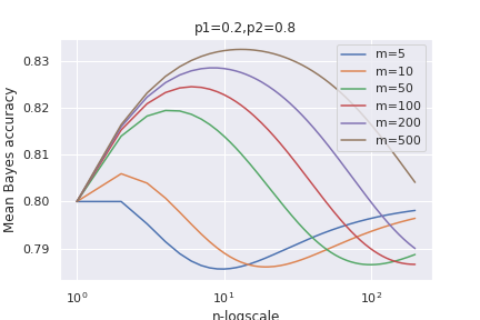
ando also for different prior probabilities:

We see that the mean accuracy first increases up to an optimal values and then it deteriorates until it reaches a limiting value for large $n$.
2. Python implementation
import matplotlib.pyplot as plt
import numpy as np
import pandas as pd
import multiprocessing as mp
import seaborn as sns
Define functions:
def term(m1,m2,s1,r1,n):
    if n==1:
        return 0
    if n==2:
        return 1
    else:
        frac=(m1-s1+n-2)/(m1+n-2)*(m2-r1+n-2)/(m2+n-2)
        return term(m1,m2,s1,r1,n-1)*frac

def f(m1,m2,s1,r1,n):
    return n*(n-1)**2*(s1+1)/((m1+n)*(m1+n-1)*(m2+n-1))*term(m1,m2,s1,r1,n)
Respectively:
\[\begin{equation*}\begin{split}&\text{term(m1,m2,s1,r1,n)}\equiv\\ & \frac{(m_1+n-s_1-2)(m_1+n-s_1-2)\ldots (m_1-s_1+1)}{(m_1+n-2)(m_1+n-3)\ldots (m_1+1)}\times (s_1\leftrightarrow r_1,m_1\leftrightarrow m_2)\end{split}\end{equation*}\]and
\[\text{f(m1,m2,s1,r1,n)}\equiv \frac{n(n-1)^2(s_1+1)}{(m_1+n)(m_1+n-1)(m_2+n-1)}\text{term(m1,m2,s1,r1,n)}\]The final expression is calculated as :
p1=0.5
p2=1-p1

def g(args):
    m1,m2,n=args
    t=0
    for r in range(m2+1):
        for s in range(r+1,m1+1):
            t+=f(m1,m2,s,r,n)*p1
    for s in range(m1+1):
        for r in range(s,m2+1):
            t+=f(m2,m1,r,s,n)*p2

    return t
Note that calculating all the sums can be computationally expensive, especially for large values of $m_1,m_2$ and $n$. We have use parallel processing to handle the calculation faster. Here is an example of how to implement this using the library multiprocessing:
data={}
m_list=[2,5,10,50,100,200,500]
for m in m_list:
    m1=int(m*p1)
    m2=m-m1
    with mp.Pool(mp.cpu_count()) as pool:
        result=pool.map(g,[(m1,m2,n) for n in range(1,100)])
    data[m]=result
References
[1] On the mean accuracy of statistical pattern recognizers, Gordon F. Hughes, “Transactions on information theory”, 1968