Linear regression classifier
1. Linear regression and classification
Suppose we have a dataset with n features and k classes. We want to fit an hyperplane. For that purpose we write the target variable $y$ in a one-hot-encoded way, that is, as a vector $y_k$ with only one entry equal to one and $k-1$ others equal zero, and fit:
\[y^k\sim w^k_{\mu}x^{\mu}+w^k_0\]where $\mu$ is the feature dimension and $w^k_0$ is the bias. Next we consider the mean square loss:
\[L=\frac{1}{m}\sum_{i=1}^{m}||(y^k_i-w^k_{\mu}x^{\mu}_i-w^k_0)||^2\]and find its minima, that is,
\[\begin{equation*}\begin{split}&\frac{\partial L}{\partial w^k_{\mu}}=-\frac{2}{m}\sum_{i=1}^{m}(y^k_i-w^k_{\nu}x^{\nu}_i-w^k_0)x^{\mu}_i=0\\ &\frac{\partial L}{\partial w^k_{0}}=-\frac{2}{m}\sum_{i=1}^{m}(y^k_i-w^k_{\mu}x^{\mu}_i-w^k_0)=0 \end{split}\end{equation*}\]Alternatively
\[\begin{equation*}\begin{split}& \langle y^kx^{\mu}\rangle-w^k_{\nu}\langle x^{\nu}x^{\mu}\rangle -w^k_0\langle x^{\mu}\rangle=0\\ &\langle y^k\rangle-w^k_{\mu}\langle x^u\rangle-w^k_0=0 \end{split}\end{equation*}\]It is best to write $w^k_a=(w^k_{\mu},w^k_0)$ and $x^{a}=(x^{\mu},1)$, so that the equations for $w^k_{\mu}$ and the bias merge into a single equation:
\[\langle y^kx^{a}\rangle-w^k_{b}\langle x^{b}x^{a}\rangle=0\]The solution is
\[w=Y^{T}X(X^{T}X)^{-1}\]where $Y=y_{ik}$ and $X=x_{ia}$. The predictor becomes:
\[\hat{Y}\equiv Xw^T=X(X^TX)^{-1}X^TY\]When is it guaranteed that there exists a solution? Or in other words, when is $X^TX$ invertible? We need to look at the vector space spanned by the columns of $X$, that is, $\text{Span}={v_a\equiv X_{ia}}$. If the dimension of this vector space is less than the number of features, then some of the vectors $v_a$ are not linearly independent, and thus the matrix $X^TX$ will have determinant zero. Or in other words, there are coefficients $c_a$ such that $\sum_ac_av_a=0$, which means that $Xc=0$ and thus $X^TXc=0$. If there are many data points as compared to the number of features, it becomes harder to find linearly dependent vectors $v_a$.
Note that
\(X^TX \Big[\begin{array}{c} 0_{\mu} \\ 1 \\ \end{array} \Big]_{a\times 1}=N\Big[\begin{array}{c} \langle x^{\mu}\rangle \\ 1 \\ \end{array} \Big]_{a\times 1}\) and therefore \(X(X^TX)^{-1}X^TY \Big[\begin{array}{c} 1_{k} \end{array}\Big]_{k\times 1}=\Big[\begin{array}{c} 1_{i} \end{array}\Big]_{i\times 1}\)
that is, the predictions $\hat{Y}_i$ sum up to one just like a probability. However, it is not guaranteed that $\hat{Y}$ is always positive. To predict the class of a datapoint we use the rule:
\[k=\text{argmax}_{k'}\hat{Y}(x)\]We can work out in more detail the inverse matrix $(X^TX)^{-1}$.
\[X^TX=N\Big[\begin{array}{cc} \langle x^{\mu}x^{\nu}\rangle & \langle x^{\mu}\rangle\\ \langle x^{\nu}\rangle & 1 \end{array}\Big]\]where $N$ is the number of datapoints. Now we use the result
\[\Big[\begin{array}{cc} A_{ij} & v_i\\ v_j & 1 \end{array}\Big]^{-1}=\Big[\begin{array}{cc} A^{-1}+\frac{A^{-1}vv^TA^{-1}}{(1-v^TA^{-1}v)} & -\frac{A^{-1}v}{(1-v^TA^{-1}v)}\\ -\frac{v^TA^{-1}}{(1-v^TA^{-1}v)} & \frac{1}{(1-v^TA^{-1}v)} \end{array}\Big]\]to find that
\[(X^TX)^{-1}=N^{-1}\Big[\begin{array}{cc} \text{Var}^{-1}_{\mu\nu} & -\sum_{\nu}\text{Var}^{-1}_{\mu\nu}\langle x^{\nu}\rangle\\ -\sum_{\mu}\langle x^{\mu}\rangle\text{Var}^{-1}_{\mu\nu}& 1+\sum_{\mu\nu}\langle x^{\mu}\rangle\text{Var}^{-1}_{\mu\nu}\langle x^{\nu}\rangle \end{array}\Big]\]where
\[\text{Var}_{\mu\nu}=\langle x^{\mu}x^{\nu}\rangle-\langle x^{\mu}\rangle \langle x^{\nu}\rangle\]is the variance matrix. On the other hand, the weight matrix $w^T$ becomes
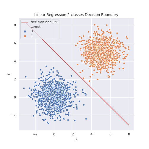
\[\Big[\begin{array}{cc} \text{Var}^{-1}_{\mu\nu} & -\sum_{\nu}\text{Var}^{-1}_{\mu\nu}\langle x^{\nu}\rangle\\ -\sum_{\mu}\langle x^{\mu}\rangle\text{Var}^{-1}_{\mu\nu}& 1+\sum_{\mu\nu}\langle x^{\mu}\rangle\text{Var}^{-1}_{\mu\nu}\langle x^{\nu}\rangle \end{array}\Big] \Big[\begin{array}{c} \langle x^{\nu}y^k\rangle\\ \langle y^k \rangle \end{array}\Big]\]Lets see how this works in practice. We build artificial data using the normal distribution in two dimensions. We consider first the case with two classes and later the multi-class case.

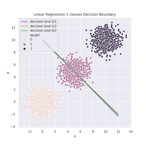
One can see that despite a very simple model the linear classifier can separate very clearly all the points. The trouble happens with more classes. Consider now the case with three classes.

We see that the linear model cannot differentiate between classes $0/1$ and $1/2$, as the decision boundaries almost overlap.
2. Python implementation
Create data (three classes)
L=1000
n1=np.random.multivariate_normal([0,0],[[1,0],[0,1]],L)
n2=np.random.multivariate_normal([5,5],[[1,0],[0,1]],L)
n3=np.random.multivariate_normal([10,10],[[1,0],[0,1]],L)

n1=np.concatenate([n1,np.zeros((L,1),int)],axis=1)
n2=np.concatenate([n2,np.ones((L,1),int)],axis=1)
n3=np.concatenate([n3,2*np.ones((L,1),int)],axis=1)

n=np.concatenate([n1,n2,n3])
data=pd.DataFrame(n, columns=['x','y','target'])
Regression:
from sklearn.linear_model import LinearRegression
from sklearn.preprocessing import OneHotEncoder

#One-hot-encoding
enc=OneHotEncoder()
Y=enc.fit_transform(data['target'].values.reshape(-1,1))

lr=LinearRegression()
lr.fit(data[['x','y']],Y.toarray())
Decision boundary:
class decision:
    def __init__(self,model):

        self.model=model

    def __call__(self,x,cl1,cl2):
        a=-(self.model.coef_[cl1]-self.model.coef_[cl2])[0]/(self.model.coef_[cl1]-self.model.coef_[cl2])[1]
        b=-(self.model.intercept_[cl1]-self.model.intercept_[cl2])/(self.model.coef_[cl1]-self.model.coef_[cl2])[1]

        return a*x+b

lr_bnd=decision(lr)

#draw line from (p1[0],p2[0]) to (p1[1],p2[1]), and so on
p1=[0,12]
p2=[lr_bnd(p1[0],0,1),lr_bnd(p1[1],0,1)]

p3=[0,12]
p4=[lr_bnd(p3[0],1,2),lr_bnd(p3[1],1,2)]

p5=[0,12]
p6=[lr_bnd(p5[0],0,2),lr_bnd(p5[1],0,2)]
Plot:
plt.figure(figsize=(7,7))
sns.scatterplot(data=data,x='x',y='y',hue='target')
plt.plot(p1,p2,linewidth=2,label='decision bnd 0/1')
plt.plot(p3,p4,linewidth=2,label='decision bnd 1/2')
plt.plot(p5,p6,linewidth=2,label='decision bnd 0/2')
plt.legend(loc='best')
plt.title('Linear Regression 3 classes Decision Boundary')
plt.show()