Logistic Regression
1. Logistic Regression
In the logistic regression algorithm the probability, of a binary class, is calculated as
\[p(c=0|x)=\sigma\Big(\sum_i \omega_i x^i +b\Big)\]where $\sigma(x)$ is the sigmoid function
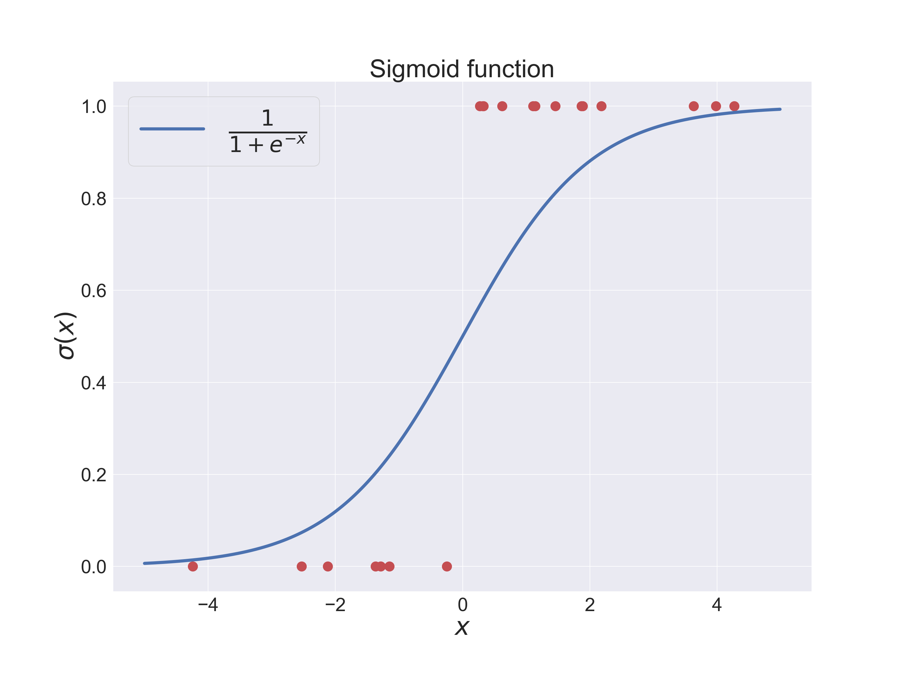
\[\sigma(z)=\frac{1}{1+e^{-z}}\]The sigmoid function approaches quickly one for large values of $z$ while it goes to zero for very negative values.

The predictor is obtained from
\[c=\text{argmax}_{c=0,1}p(c|x)\]The red dots in the picture above represent a few examples.
The logistic function is composed of a linear followed by a non-linear operation, given by the sigmoid function. This composed operation is usually represented in the diagram

where $x^i$ are the features of the datapoint $x$. The node (circle) represents the composition of a linear operation followed by a non-linear function. In more complex graphs, the sigmoid function’s output can become the input of an additional non-linear operation. This way, we can stack various non-linear operations, which give an increased level of complexity. This type of graph has the name of neural network.
In the multiclass case, the probabilities have instead the form
\[p(y^k|x)=\frac{e^{z^k(x)}}{Z(x)}\]where $z^k=-\sum_i\omega^k_i x^i-b^k$ and $Z(x)=\sum_l e^{z^l(x)}$ is a normalization. Diagrammatically this has the form

where the function
\[f(z)^k=\frac{e^{z^k}}{\sum_l e^{z^l}}\]is the softmax function. It provides with a non-linear operation after the linear transformation $z^k=-\omega^k_ix^i-b$. Since the softmax function is invariant under $z^k\rightarrow z^k+\lambda$, we can choose to fix $z^0$ to zero, which implies $\omega^0_i=0$ and $b^0=0$.
Given a dataset $S={(\vec{x}_0,y_0),(\vec{x}_1,y_1),\ldots (\vec{x}_N,y_N)}$ we determine the parameters $\omega$ and $b$ using maximum-likelihood estimation, that is, we minimize the loss function
\[\begin{equation*}\begin{split}\mathcal{L}=&-\frac{1}{N}\sum_{i=1}^N \ln p(y^i|\vec{x}_i)\\ =&\frac{1}{N}\sum_i \omega^i_jx^j+b^i+\ln Z(\vec{x}_i)\end{split}\end{equation*}\]One of the main advantages of using the logistic function is that it makes the loss function convex, which allows us to apply more robust optimization algorithms like the Newton-Raphson method. To see that the loss function is convex, lets for simplicity define $\omega^k\equiv(\omega^k_i,b^k)$ and $x\equiv(x^i,1)$. Calculating the derivatives of the loss function
\[\frac{\partial \mathcal{L}}{\partial \omega^{\mu}_{\nu}}=\langle \delta^k_{\mu}x^{\nu}\rangle_{y^k,x}-\langle x^{\nu}p_{\mu}(x)\rangle_{x}\]where $p_{\mu}(x)$ is the probability, $\delta$ is the Kroenecker delta function, and $\langle \rangle$ represents sample averages. And the second derivatives
\[\frac{\partial^2 \mathcal{L}}{\partial \omega^{\mu}_{\nu} \partial \omega^{\alpha}_{\beta}}=\langle x^{\nu}x^{\beta}\delta_{\mu\alpha}p_{\mu}(x) \rangle_x -\langle x^{\nu}x^{\beta}p_{\mu}(x)p_{\alpha}(x) \rangle_x\]To show this is a convex optimization problem, we build the quadratic polynomial in $\lambda^{\mu}_{\nu}$ at a point $x$,
\[\begin{equation*}\begin{split}&\sum_{\mu,\nu,\alpha,\beta}x^{\nu}x^{\beta}\delta_{\mu\alpha}p_{\mu}(x)\lambda^{\mu}_{\nu}\lambda^{\alpha}_{\beta}-x^{\nu}x^{\beta}p_{\mu}(x)p_{\alpha}(x)\lambda^{\mu}_{\nu}\lambda^{\alpha}_{\beta}=\\ &\sum_{\mu} p_{\mu}(x)(\lambda^{\mu}_{\nu}x^{\nu})^2-\Big(\sum_{\mu}p_{\mu}(x)\lambda^{\mu}_{\nu}x^{\nu}\Big)^2=\langle \lambda^2\rangle-\langle \lambda\rangle^2\geq 0\end{split}\end{equation*}\]Summing over $x$ we show that
\[\sum_{\mu,\nu,\alpha,\beta}\frac{\partial^2 \mathcal{L}}{\partial \omega^{\mu}_{\nu} \partial \omega^{\alpha}_{\beta}} \lambda^{\mu}_{\nu}\lambda^{\alpha}_{\beta}\geq 0\]2. Newton-Raphson method
The Newton-Raphson method provides with a second-order optimization algorithm. In essence it consists in solving iteratively a second-order expansion of the loss function. First, we Taylor expand the loss function to second order
\[\mathcal{L}=\mathcal{L}(\omega_0)+\frac{\partial \mathcal{L}}{\partial\omega_i}|_{\omega_0}\Delta\omega_i+\frac{1}{2}\frac{\partial^2 \mathcal{L}}{\partial\omega_i\partial\omega_j}|_{\omega_0}\Delta\omega_i\Delta\omega_j+\mathcal{O}(\Delta\omega^3)\]Then we solve for $\Delta\omega$
\[\Delta\omega=\text{argmin}\frac{\partial \mathcal{L}}{\partial\omega_i}|_{\omega_0}\Delta\omega_i+\frac{1}{2}\frac{\partial^2 \mathcal{L}}{\partial\omega_i\partial\omega_j}|_{\omega_0}\Delta\omega_i\Delta\omega_j\]that is,
\[\Delta\omega_i=-\sum_j\Big(\frac{\partial^2 \mathcal{L}}{\partial\omega_i\partial\omega_j}|_{\omega_0}\Big)^{-1}\frac{\partial \mathcal{L}}{\partial\omega_j}|_{\omega_0}\]The algorithm consists of updating the reference point $\omega_0$ as
\[\omega_0\rightarrow \omega_0+\Delta\omega\]and continuing iteratively by solving the derivatives on the new reference point. In the logistic regression case, the parameter $\omega_i$ is a matrix with components $\omega^k_i$. Determining the inverse of a $n\times n$ matrix is an order $\mathcal{O}(n^3)$ (with Gaussian elimination) process, while the matrix-vector multiplication operations are of order $\mathcal{O}(n^2)$. Therefore each step of the Newton-Raphson method is a $\mathcal{O}(n^3)$ process. Since $n=K(d+1)$ where $K$ is the number of classes and $d$ is the feature dimension, the Newton-Raphson is a fast algorithm provided both $K$ and $d$ are relatively small.
3. Decision Boundary
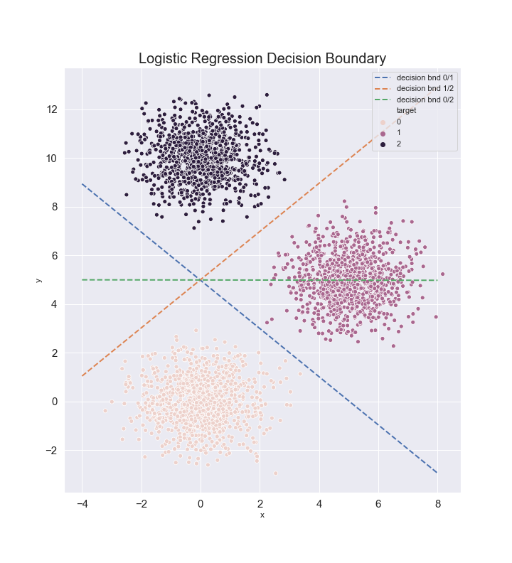
In a binary classification problem the decision boundary of the logistic regression is a hyperplane. This is because the threshold value $p(0|x)=0.5$ implies the linear constraint $\sum_i\omega_i x^i+b=0$. For more classes, the decision boundary corresponds to regions bounded by hyperplanes. For any two classes $c_1,c_2$ we determine a pseudo-boundary, that is, the hyperplane represented by the equation $p(c_1|x)=p(c_2|x)$. This gives
\[\text{hyperplane}_{c_1,c_2}:\;\sum_i(\omega^{c_1}_i-\omega^{c_2}_i)x^i+b^{c_1}-b^{c_2}=0\]For $N$ classes we have $N(N-1)/2$ hyperplanes. We can use these hyperplanes to determine the predicted class. For example, in two dimensions

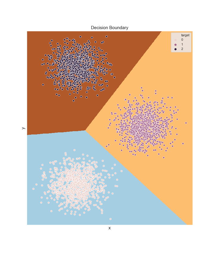
We can show that the regions for the predicted classes are simply connected convex sets. Consider two points $x_1$ and $x_2$, both belonging to the same predicted class $k$. We construct the set
\[(1-\lambda)x_1+\lambda x_2,\;0\leq\lambda\leq 1\]Since $\sum_i\omega^k_ix^i_1+b^k\geq \sum_i\omega^{j}_i x^i_1+b^j,\;j\neq k$ and similarly for $x_2$, we must have
\[(1-\lambda)\sum_i\omega^k_ix^i_1+\lambda \sum_i\omega^k_ix^i_2+b^k\geq (1-\lambda)\sum_i\omega^j_ix^i_1+\lambda \sum_i\omega^j_ix^i_2 +b^j,\;j\neq k\]since $\lambda\geq 0$ and $1-\lambda\geq 0$. This means that all the points belonging to the set connecting $x_1$ and $x_2$ have the same class, which thus implies that the region with predicted class $k$ must be singly connected, and convex. For example, for the data above

4. Python Implementation
# class ProbSoftmax is the model
class ProbSoftmax:
    def __init__(self,n_features,n_classes):
        self.n_features=n_features
        self.n_classes=n_classes
        self.weight=np.random.normal(0,0.1,(n_classes,n_features))
        self.weight[0]=0

    def __call__(self,x):

        wx=-np.dot(x,self.weight.T)
        wx=np.exp(wx)
        Z=wx.sum(1).reshape(-1,1)
        return wx/Z
Optimizer class with backward and step methods:
# class logloss calculates the loss function and the Newton-Raphson step.
class logloss:
    def __init__(self,model):

        self.prob=model #model: ProbSoftmax object
        self.delta_w=None
        self.nf=model.n_features
        self.nc=model.n_classes

    def backward(self,x,y):
        p=self.prob(x)
        z=np.tensordot(x,y[:,1:]-p[:,1:],axes=[0,0])
        z=z.reshape(-1,1)
        z=z/x.shape[0]

        return z

    def back_square(self,x):
        p=self.prob(x)
        p=p[:,1:]

        z=0
        for a,b in zip(x,p):
            idt=np.diag(b)
            k=np.outer(a,a)
            w=np.outer(b,b)
            z+=np.tensordot(k,idt-w,axes=0)
        z=np.transpose(z,(0,2,1,3))
        z=z.reshape(z.shape[0],z.shape[1],z.shape[2]*z.shape[3])
        z=z.reshape(z.shape[0]*z.shape[1],-1)
        z=z/x.shape[0]

        return z

    def step(self):

        self.prob.weight[1:,:]+=self.delta_w

    def delta(self,x,y):

        f=self.backward(x,y)
        M=self.back_square(x)
        M_inv=np.linalg.inv(M)
        delta_w=-np.dot(M_inv,f)
        delta_w=delta_w.reshape(self.nf,-1)
        delta_w=delta_w.T
        return delta_w

    def __call__(self,x,y):
        #y is hot encoded
        p=self.prob(x)
        p=p*y
        p=p.sum(1)
        self.delta_w=self.delta(x,y)

        return -np.log(p).mean()
Training function:
def training(model,x,y,num_iter=10):
    loss=logloss(model)
    for i in range(num_iter):
        L=loss(x,y) #when calling, the object calculates the derivatives and determines the Newton-Raphson step
        loss.step() #it shifts w by delta_w
        print("Loss=",L," iter:",i)