Linear Discriminant Analysis
- 1. LDA
- 2. Decision Boundary
- 3. Dimensionality Reduction
- 4. Quadratic Discriminant Analysis
- 5. Python Implementation
1. LDA
The LDA or linear discriminant analysis is an algorithm whereby the probability has the following form
\[p(x|c)=\frac{1}{\sqrt{(2\pi)^d\text{det}(\Sigma)}}e^{-\frac{1}{2}(x-\mu_c)^t\Sigma^{-1}(x-\mu_c)}\]where $c$ is the class and $p(c)=\pi_c$. Using Bayes theorem we calculate
\[p(c|x)=\frac{p(x|c)\pi_c}{\sum_k p(x|k)\pi_k}=\frac{e^{-\frac{1}{2}(x-\mu_c)^t\Sigma^{-1}(x-\mu_c)}\pi_c}{\sum_k e^{-\frac{1}{2}(x-\mu_k)^t\Sigma^{-1}(x-\mu_k)}\pi_k}=\frac{e^{-\mu_c^t\Sigma^{-1}x-\frac{1}{2}\mu_c^t\Sigma^{-1}\mu_c }\pi_c}{\sum_ke^{-\mu_k^t\Sigma^{-1}x-\frac{1}{2}\mu_k^t\Sigma^{-1}\mu_k }\pi_k}\]Note that this has precisely the form of the logistic regression probability. We can conclude right away that the predicted classes form simply connected convex sets. However, to train the LDA algorithm we use instead the probability \(p(x,c)\) rather than $p(c|x)$ as in the logistic case. We proceed as usual by minimizing the log loss function
\[\begin{equation*}\begin{split}\mathcal{L}&=-\sum_i \ln p(x_i,c_i)\\ &=-\sum_i \ln(\pi_{c_i}) +\sum_i \frac{1}{2}(x_i-\mu_{c_i})^t\Sigma^{-1}(x_i-\mu_{c_i})+\frac{N}{2}\ln\text{det}(\Sigma)+\frac{Nd}{2}\ln(2\pi)\end{split}\end{equation*}\]Using the property
\[\frac{\partial}{\partial \Sigma^{-1}_{ij}}\ln\text{det}\Sigma=-\Sigma_{ij}\]we calculate
\[\frac{\partial}{\partial \Sigma^{-1}_{ij}}\mathcal{L}=0\iff \Sigma_{ij}=\frac{1}{N}\sum_k(x_k-\mu_{c_k})_i(x_k-\mu_{c_k})_j\]While the other parameters are calculated as
\[\frac{\partial}{\partial \mu_c}\mathcal{L}=0\iff \frac{1}{N_c}\sum_{k: y=c} x_k\]where the sum is over the $N_c$ datapoints with class $c$, and
\[\frac{\partial}{\partial \pi_c}\mathcal{L}=0\iff \pi_c=\frac{N_c}{N}\]2. Decision Boundary
The predictor is determined by the maximum of \(p(c|x)\) . As we have seen above, this probability has the same form as the logistic regression. This means that also, for LDA, the regions of the predicted class are singly connected convex sets.
3. Dimensionality Reduction
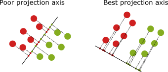
The PCA, or principal component analysis, is an algorithm that reduces the dimensionality of the dataset while keeping the most relevant features. However, the PCA analysis does not discriminate over the classes, which may lead to a lack of predictability in supervised learning problems. The right projection keeps the classes separated in the example below, which is a better projection than the one on the left.

Besides being a Gaussian classifier, the LDA can be used to reduce the data dimensionally. The basic idea is to find a projection axis that maximizes the “between” class variance while, at the same time, minimizes the “within” class variance. That is, we make the gaussians more narrow, and at the same time, the centers become farther apart from each other.
Consider the covariance matrix given by
We can write this as
\[\begin{equation*}\begin{split}\sum_x (x_i-\bar{x}_i)(x_j-\bar{x}_j)&=\sum_c\sum_{x\in \text{class }c} (x_i-\bar{x}_i)(x_j-\bar{x}_j)\\ &=\sum_c\sum_{x\in \text{class }c}(x_i-\bar{x}^c_i)(x_j-\bar{x}^c_j)+\sum_c N_c(\bar{x}^c_i-\bar{x}_i)(\bar{x}^c_j-\bar{x}_j)\end{split}\end{equation*}\]where $\bar{x}^c$ is the average of $x$ within class $c$ and $N_c$ is the number of points in class $c$. The first term above is known as “within” class covariance, which we denote as $\textbf{W}$, and the second term as “between” class covariance, denoted as $\textbf{B}$. We want to maximize the quotient
\[\text{max}_v\frac{v^T\textbf{B}v}{v^T\textbf{W}v}\]For that purpose we consider the eigenvalues $\lambda$ and eigenvectores $v_{\lambda}$ of $\textbf{W}^{-1}\textbf{B}$. The quotient becomes
\[\frac{v_{\lambda}^T\textbf{W}\textbf{W}^{-1}\textbf{B}v_{\lambda}}{v_{\lambda}^T\textbf{W}v_{\lambda}}=\lambda\]It is easy to show that the stationary directions of the quotient correspond to the eigen-directions. Hence the direction of best projection is along the eigenvector with largest eingenvalue.
4. Quadratic Discriminant Analysis
In QDA or quadratic discriminant analysis the covariance matrix is not necessarily constant across the various classes, instead we have
\[p(x|c)=\frac{1}{\sqrt{(2\pi)^d\text{det}(\Sigma_c)}}e^{-\frac{1}{2}(x-\mu_c)^t\Sigma_c^{-1}(x-\mu_c)}\]This means that the likelihood $p(c|x)$ now depends on the covariance matrix, that is,
\[p(c|x)=\frac{p(x|c)\pi_c}{\sum_k p(x|k)\pi_k}=\frac{1}{\sqrt{(2\pi)^d\text{det}(\Sigma_c)}}\frac{e^{-\frac{1}{2}(x-\mu_c)^t\Sigma_c^{-1}(x-\mu_c)}\pi_c}{\sum_k p(x|k)\pi_k}\]5. Python Implementation
class LDAmodel:

    def __init__(self,sigma=None,mu=None,prior_prob=None):
        self.sigma=sigma
        self.mu=mu
        self.prior_prob=prior_prob
        if sigma is None:
            self.inv=None
            self.det=None
        else:
            self.inv=np.linalg.inv(sigma)
            self.det=np.linalg.det(sigma)
        if mu==None:
            self.nc=None
            self.dim=None
        else:
            self.nc=mu.shape[0]
            self.dim=mu.shape[1]

        self.coef_=None
        self.intercept_=None

    def means(self,x,y):
        yset=set(y)
        means=np.zeros((len(yset),x.shape[1]))
        for i in yset:
            means[i]=x[y==i].mean(0)
        return means

    def var(self,x,y):
        yset=set(y)
        d=x.shape[1]
        var=np.zeros((d,d))
        means=self.means(x,y)
        for i in yset:
            c=x[y==i]-means[i]
            var+=np.tensordot(c,c,axes=[0,0])
        var=var/x.shape[0]

        return var

    def priors(self,x,y):
        priors=np.zeros(3)
        yset=set(y)
        for i in yset:
            priors[i]=(y==i).sum()/y.shape[0]

        return priors

    def fit(self,x,y):
        self.mu=self.means(x,y)
        self.sigma=self.var(x,y)
        self.prior_prob=self.priors(x,y)
        self.inv=np.linalg.inv(self.sigma)
        self.det=np.linalg.det(self.sigma)
        self.nc=len(set(y))
        self.dim=x.shape[1]

        self.coef_=np.dot(self.mu,self.inv)
        self.intercept_=np.zeros(self.nc)
        for i in range(self.nc):
            v=np.dot(self.inv,self.mu[i])
            self.intercept_[i]=-0.5*np.dot(self.mu[i],v)

    def __call__(self,x):
        probs=np.zeros((x.shape[0],self.nc))
        for i in range(self.nc):
            t=x-self.mu[i]
            w=np.dot(t,self.inv)
            w=(t*w).sum(1)
            probs[:,i]=np.exp(-0.5*w)*self.priors[i]
            probs[:,i]=probs[:,i]/((2*np.pi)**(self.dim/2)*np.sqrt(np.abs(self.det)))
        Z=probs.sum(1)
        return probs/Z.reshape(-1,1)