Gradient Boosting
1. Gradient boosting
In gradient boosting, much like in adaboost, we fit a sequence of weak learners in an iterative manner. In this way, the predictor at the mth-step is given as a sum of the predictors from previoues iterations, that is,
\[F_m(x)=\gamma_0+\gamma_1 w_1(x)+\ldots+\gamma_m w_m(x)\]where $w_i(x)$ is the weak-learner predictor and $\gamma_0$ is a constant.
To motivate the gradient we consider the Taylor approximation of the loss function around $F_{m-1}$, that is,
\[L(F_m)=L(F_{m-1})+\frac{\partial L}{\partial F}\Bigr|_{F_{m-1}}(F_m-F_{m-1})+\ldots\]In the gradient descent algorithm we take a step of magnitude proportional to
\[F_m-F_{m-1}\propto-\frac{\partial L}{\partial F_{m-1}}\]The constant of proportionality is the learning rate. Since
\[F_m-F_{m-1}\propto w(x)\]the best we can do is to fit $w(x)$ to the gradient descent direction, that is,
\[w(x)\sim -\frac{\partial L}{\partial F_{m-1}}\]where $\sim$ means that we fit the learner. In order to fix $\gamma_m$, effectively the learning rate, we solve the one-dimensional optimization problem
\[\gamma_m=\text{argmin}_{\gamma_m} L(y,F_{m-1}+\gamma_m w(x))\]where $y$ is the target array. We repeat this process until the solution is sufficiently accurate.
To exemplify how this works in practice, consider a binary classification problem. In this case, we use the logit function using the boosting algorithm. In other words, we assume that the likelihood \(p(y=0|x)\) has the form
\[p(y=0|x)=\frac{1}{1+e^{-F_m(x)}}\]with $F_m(x)$ given as above. The loss $L$ is the the log-loss function. The gradient descent direction is given by the variational derivative, that is,
\[r^i\equiv-\frac{\partial L}{\partial F_{m-1}}\Bigr|_{x^i}=\frac{e^{-F_{m-1}(x^i)}}{1+e^{-F_{m-1}(x^i)}}-y^i\]and we fit $w_m(x)$ to $r^i$. Then we are left with the minimization problem
\[\text{argmin}_{\gamma_m} \sum_{y^i=0}\ln\Big( 1+e^{-F_{m-1}(x^i)-\gamma_m w_m(x^i)}\Big) -\sum_{y^i=1}\ln \Big(\frac{e^{-F_{m-1}(x^i)-\gamma_m w(x^i)}}{1+e^{-F_{m-1}(x^i)-\gamma_m w(x^i)}}\Big)\]which determines the learning rate, that is, $\gamma_m$. This is a convex optimization problem and can be solved using the Newton-Raphson method.
2. Decision Boundary
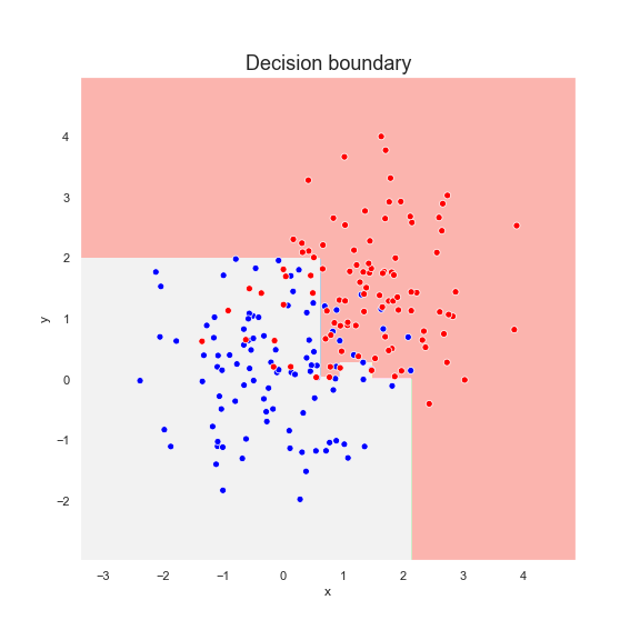
We fit an GradBoost classifier to a dataset consisting of two sets of points, red and blue, which are normally distributed. Below is the Gradient boosting prediction after six steps.

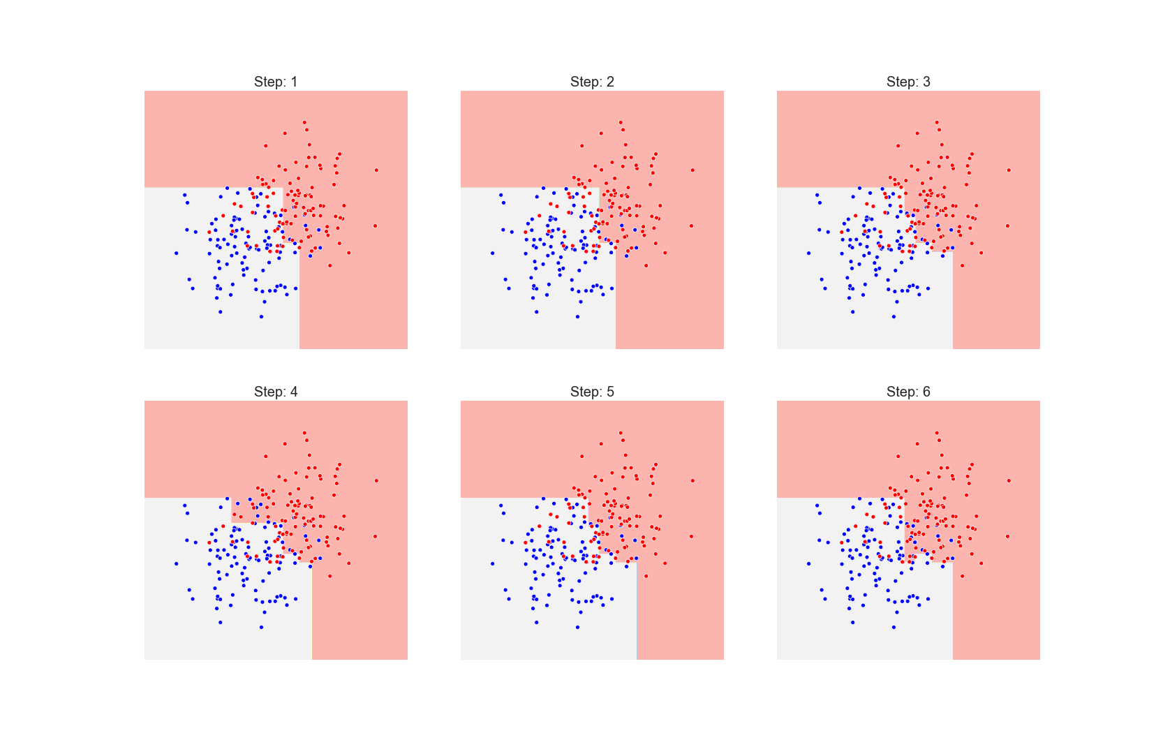
And below we present the prediction at each step of training, from left to right

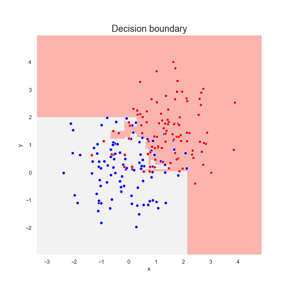
One can see that the algorithm is trying to overfit the data by drawing a more complex decision boundary at each step. If we let the algorithm run with 30 estimators the decision boundary becomes very complex

3. Python implementation
The class node encapsulates the data structure that we will use to store fitted models.
class node:
    def __init__(self,tree=None,gamma=None):
        self.tree=tree
        self.gamma=gamma
        self.next=None

    def insert(self,tree,gamma):

        if self.next is None:
            self.next=node(tree,gamma)
        else:
            return self.next.insert(tree,gamma)

    def output(self,x):
        if self.tree is not None:
            out=self.tree.predict(x)
        if self.next is None:
            return out*self.gamma
        else:
            return out*self.gamma+self.next.output(x)
The GradBoostClassifier class implements the boosting algorithm. We use the Newton-Raphson method to determine $\gamma$ at each step in the iteration.
class GradBoostClassifier:
    def __init__(self,n_iter):
        self.n_iter=n_iter
        self.head=None
        self.classes=None
        self.gamma0=None

    def __sigmoid(self,x):
        prob=np.exp(x)/(1+np.exp(x))

        return prob

    def __minima(self,h,F,y):
        g=0.1
        g_prev=0.1
        cl=self.classes[0]

        not_converged=True
        i=0
        while not_converged:
            prob=self.__sigmoid(F+g*h)
            grad_dd=h*h*p*(1-p)
            grad_dd=grad_dd.sum()
            grad_d=h*(p-y)
            grad_d=grad_d.sum()

            delta=-grad_d/grad_dd
            g+=delta
            i+=1
            if np.abs(g_prev-g)<0.01:
                not_converged=False
            if i>10000:
                break
            g_prev=g

        return g

    def fit(self,x,y):
        self.head=node()
        self.classes=sorted(list(set(y)))
        self.class_dic={c:i for i,c in enumerate(self.classes)}
        cl=self.classes[0]

        yc=y.copy()
        yc[y==cl]=0
        yc[y!=cl]=1
        n1=(yc==1).sum()
        n0=(yc==0).sum()
        self.gamma0=np.log(n1/n0)

        #1st STEP
        F=self.gamma0
        p=n1/(n1+n0)*np.ones(x.shape[0])
        res=-p+yc
        tree=DecisionTreeRegressor(max_depth=3)
        tree.fit(x,res)
        h=tree.predict(x)
        gamma=self.__minima(h,F,yc)
        self.head.tree=tree
        self.head.gamma=gamma

        for i in range(1,self.n_iter):
            F=self.gamma0+self.head.output(x)
            p=self.__sigmoid(F)
            res=-p+yc
            tree=DecisionTreeRegressor(max_depth=3)
            tree.fit(x,res)
            h=tree.predict(x)
            gamma=self.__minima(h,F,yc)
            self.head.insert(tree,gamma)

    def predict(self,x):
        p=self.gamma0+self.head.output(x)
        p=self.__sigmoid(p)
        ycl=(p>=0.5).astype(int)
        ypred=ycl.copy()
        ypred[ycl==1]=self.classes[1]
        ypred[ycl==0]=self.classes[0]

        return ypred

    def predict_prob(self,x):
        p=self.gamma0+self.head.output(x)
        p=self.__sigmoid(p)
        return p