Recurrent Neural Network
1. RNN architecture
A recurrent neural network (RNN) learns sequential data. For example, text is a type of sequential data because a character depends on their previous neighbors in order of appearance. Similarly, for the sequence of words themselves.
Suppose we want to study a sequence of data \(x_{0},x_{1},\ldots x_{t}\). Given this data, we want to model the probability of finding \(x_{t+1}\). That is, we want to calculate
\[P(x_{t+1}|x_{t},\ldots,x_0)\]Using the chain rule, we can write the probability of finding the full sequence as
\[P(x_{0},\ldots,x_{t},x_{t+1})=P(x_{t+1}|x_{t},\ldots, x_0)P(x_{t}|x_{t-1},\ldots,x_0)\ldots P(x_{1}|x_0)P(x_0)\]If we write \(h_t\) to denote all the previous states up to time \(t-1\)
\[h_t\equiv \{x_0,x_1\ldots x_{t-1}\}\]then the probability becomes
\[P(x_{0},\ldots,x_{t},x_{t+1})=P(x_{t+1}|x_t,h_t)P(x_t|x_{t-1},h_{t-1})\ldots P(x_1|x_0,h_0)\]The hidden variable \(h_t\) lives in a space we have yet to determine. Because the probability is now the product of the probabilities at each time \(t\), the loss function (using maximum likelihood) is,
\[L=-\sum_t \ln P(x_t|x_{t-1},h_{t-1})\]where the sum runs over all the elements in the sequence. Below is depicted a recurrent neural network unit that models the probability \(P(x_{t+1}|x_t,h_t)\):
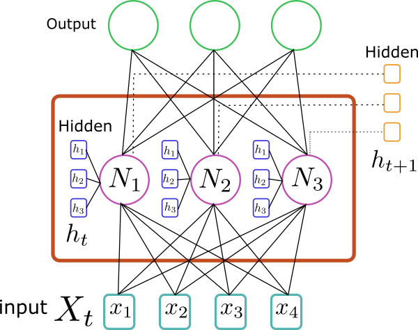
Each node \(N_i\) contains an activation unit that takes the input \(x_t\) and the hidden state \(h_t\). That is, for each node \(N_i\) one calculates
\[h_{t+1}^i=g(\sum_jW^x_{ij}x_t^j+\sum_{\alpha}W^h_{i\alpha}h^{\alpha}_t+b_i)\]where \(W^x, W^h, b\) are the parameters we want to fit. The resulting hidden state \(h_{t+1}\) sequentially passes to the next unit. To determine the probability, we stack a softmax layer on top of the hidden layer, that is,
\[P(x_{t+1}|x_t,h_t)=\frac{e^{\sum_iw_{ai}h_{t+1}^i+\tilde{b}_a}}{\sum_a e^{\sum_i w_{ai}h_{t+1}^i+\tilde{b}_a}}\]where \(a\) is the class of \(x_{t+1}\).
We can include additional hidden layers, and they can have a different number of nodes. At each step, we have a set of ingoing hidden states \(h^1,h^2,\ldots\) for the layers 1,2, etc, and an outgoing set of hidden states.
2. Training
Training a full sequence of data can be problematic. The gradients depend on all the past units, which for a long series makes the problem computationally very expensive. Due to the backpropagation algorithm the gradients contain many products that may lead the gradient to explode or become extremely small. Instead, we can divide the full sequence into shorter sequences. We feed the algorithm using batches of size \(N\) with sequences of length \(L\). We can stack several units horizontally, so we have a single network acting on a series.
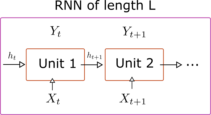
Here \(Y\) stands for the target.
The backpropagation algorithm acquires a component along the time direction. Say we want to calculate the derivative of the loss function with respect to \(\omega\), the parameter that multiplies \(x_0\). Then the gradient will receive several contributions coming from the later units because of the recurrence relationship.
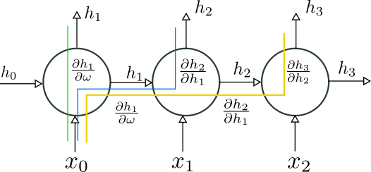
In this example we have
\[\begin{equation*}\begin{split}\frac{\partial L}{\partial \omega}&=\frac{\partial L_1}{\partial h_1}\frac{\partial h_1}{\partial \omega}+\frac{\partial L_2}{\partial h_2}\frac{\partial h_2}{\partial \omega}+\frac{\partial L_3}{\partial h_3}\frac{\partial h_3}{\partial \omega}+\ldots\\ &+\frac{\partial L_2}{\partial h_2}\frac{\partial h_2}{\partial h_1}\frac{\partial h_1}{\partial \omega}+\frac{\partial L_3}{\partial h_3}\frac{\partial h_3}{\partial h_2}\frac{\partial h_2}{\partial \omega}+\ldots\\ &+\frac{\partial L_3}{\partial h_3}\frac{\partial h_3}{\partial h_2}\frac{\partial h_2}{\partial h_1}\frac{\partial h_1}{\partial \omega}+\ldots\end{split}\end{equation*}\]where \(L_i\) is the contribution to the loss function coming from the i-th term in the sequence. More generally, we calculate
\[\begin{equation*}\begin{split}\frac{\partial L}{\partial \omega}&=\sum_i \frac{\partial L_i}{\partial h_i}\frac{\partial h_i}{\partial \omega}+\sum_i\frac{\partial L_{i+1}}{\partial h_{i+1}}\frac{\partial h_{i+1}}{\partial h_i}\frac{\partial h_i}{\partial \omega} + \sum_i\frac{\partial L_{i+2}}{\partial h_{i+2}}\frac{\partial h_{i+2}}{\partial h_{i+1}}\frac{\partial h_{i+1}}{\partial h_i}\frac{\partial h_i}{\partial \omega}+\ldots\\ &=\sum_n \sum_i \frac{\partial L_{i+n}}{\partial h_{i+n}}\frac{\partial h_i}{\partial \omega}\prod_{j=i}^{n-1+i} \frac{\partial h_{j+1}}{\partial h_{j}} \end{split}\end{equation*}\]3. Python Implementation
For this implementation, we consider a one-dimensional input \(x\) and hidden state \(h\) with dimension \(d\). For the activation function we take the \(\tanh\) function. So in each unit we have
\[h_{t+1,i}=\tanh(w^0_ix_t+w^1_{ij}h^j_t+b^0_{t,i})\]and we calculate the derivatives
\[\begin{equation*}\begin{split}&\frac{\partial h_{t+1,i}}{\partial h_{t,j}}=(1-h_{t+1,i}^2)w^1_{ij}\\ &\frac{\partial h_{t+1,i}}{\partial w^1_{ij}}=(1-h_{t+1,i}^2)h_{t,j}\\ &\frac{\partial h_{t+1,i}}{\partial w^0_i}=(1-h_{t+1,i}^2)x_t\\ &\frac{\partial h_{t+1,i}}{\partial b^0_{t,i}}=(1-h_{t+1,i}^2)\end{split}\end{equation*}\]We consider a regression problem, and as such the predictor has the form
\[\hat{y}_{t+1,a}= w^2_{ai} h_{t+1,i}+b^1_{t,a}=w^2_{ai} \tanh(w^0_ix_t+w^1_{ij}h_{t,j}+b^0_{t,i}) + b^1_{t,a}\]where the target has features \(a\).
From the loss function \(L=\sum_t L_t=\frac{1}{2N}\sum_{t=1}^N (y_t-\hat{y}_t)^2\)
we calculate \(\frac{\partial L_t}{\partial h_{t,i}}=\frac{1}{N}(\hat{y}_t-y_t)_aw^2_{ai}\)
We define classes for the recurrent neural network, loss function and optimizer, that implements, the gradient descent update.
class LinearLayer:
    def __init__(self,input_dim,out_dim,bias=True):
        self.weight=np.random.rand(input_dim,out_dim)
        if bias:
            self.bias=np.random.rand(out_dim)
        else:
            self.bias=0

    def __call__(self,x):
        out=np.matmul(x,self.weight)+self.bias
        return out

class RNN:
    def __init__(self,input_dim,hidden_dim,out_dim):
        self.hidden_dim=hidden_dim
        self.input_dim=input_dim
        self.out_dim=out_dim

        self.out_layer=LinearLayer(hidden_dim,out_dim)
        self.wx=LinearLayer(input_dim,hidden_dim,bias=False)
        self.wh=LinearLayer(hidden_dim,hidden_dim,bias=False)
        self.bias=np.random.rand(hidden_dim)
        self.g=np.tanh

        self.gradients=None
        self.cache=None

        self.parameters={'dh_dwh':self.wh.weight,
                         'dh_dwx':self.wx.weight,
                         'dh_db':self.bias,
                         'dw2':self.out_layer.weight,
                         'db2':self.out_layer.bias}

    def __call__(self,x):
        hidden=np.zeros(self.hidden_dim)
        h=np.zeros((x.shape[0],self.hidden_dim))

        for i,xi in enumerate(x):
            h[i]=self.g(self.wx(xi)+self.wh(hidden)+self.bias)
            hidden=h[i]


        out=self.out_layer(h)
        self.cache={'hidden':h,'output':out}

        return out

    def grads(self,x,h_t,h_tp1):
        mat=np.identity(self.hidden_dim)
        np.fill_diagonal(mat,1-h_tp1*h_tp1)

        dh_dwh=np.tensordot(mat,h_t,axes=0) #[hid_dim,hid_dim,hid_dim]
        dh_dwx=np.tensordot(mat,x,axes=0) #[hid_dim,hid_dim,input_dim]
        dh_dh=np.dot(mat,self.wh.weight) #[hid_dim,hid_dim]
        dh_db=mat #[hid_dim,hid_dim]

        return dh_dh, {'dh_dwh':dh_dwh,'dh_dwx':dh_dwx,'dh_db':dh_db}
The mean-square loss function:
class MSE_Loss:
    def __init__(self,model):
        self.model=model

    def __call__(self,x,y):
        y_pred=self.model(x)
        loss=y-y_pred
        loss=loss*loss

        return loss.mean()

    def backward(self,x,y):

        L=x.shape[0]
        h=self.model.cache['hidden']
        out=self.model.cache['output']
        z=(out-y)/L # (y_pred-y)/N

        w2=self.model.out_layer.weight.T #[out_dim,hidden_dim]
        grads_cache={'dh_dwh':[],'dh_dwx':[],'dh_db':[]}
        grads_total={'dh_dwh': 0,'dh_dwx': 0,'dh_db': 0}

        hidden=np.zeros(self.model.hidden_dim)
        for i,xi in enumerate(x):

            dh_dh,grads=self.model.grads(xi,hidden,h[i])
            hidden=h[i]

            for var,grad in grads.items():
                wt=np.dot(w2,grad)
                grads_cache[var].append(grad)
                grads_total[var]+=np.tensordot(z[i],wt,axes=([0],[0]))

            if i>0:
                for var in grads_cache.keys():
                    temp=[]
                    for j, dh in enumerate(grads_cache[var]):
                        wt=np.tensordot(dh_dh,dh,axes=([1],[0]))
                        temp.append(wt)
                        wt2=np.tensordot(w2,wt,axes=([1],[0]))
                        a=np.tensordot(z[i],wt2,axes=([0],[0]))
                        grads_total[var]+=a

                    grads_cache[var]=temp[:]

        grads_total['dw2']=np.tensordot(z,h,axes=([0],[0])).T
        grads_total['db2']=z.sum(0)
        grads_total['dh_dwh']=grads_total['dh_dwh'].T
        grads_total['dh_dwx']=grads_total['dh_dwx'].T

        self.model.gradients=grads_total
the optimizer
class Optimizer:
    def __init__(self,model,lr):
        self.model=model
        self.lr=lr

    def step(self):
        grads=self.model.gradients

        for var in self.model.parameters:
            self.model.parameters[var]-=self.lr*grads[var]
and the training function:
def train(seqs,targets,model, loss,optimizer,epochs):

    for epoch in range(epochs):
        total_loss=0
        for seq,target in tqdm(zip(seqs,targets),total=len(seqs)):
            ypred=model(seq)
            total_loss+=loss(ypred,target)
            loss.backward(seq,target)
            optimizer.step()

        print('epoch: ',epoch,' Loss: ',total_loss)
Data preparation:
seq_len=10
seqs=[]
targets=[]
xs=[]
for n in range(100):
    ts=np.linspace(n*np.pi,(n+1)*np.pi,seq_len+1)
    xs.append(ts[:-1])
    data=np.sin(ts)
    # add noise
    data=data.reshape(-1,1)
    noise=np.random.normal(0,0.008,data.shape)
    data+=noise

    seqs.append(data[:-1])
    targets.append(data[1:].reshape(-1,1))
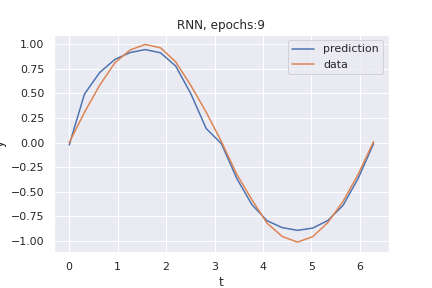
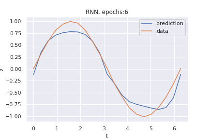
This is the result of training after only 6 epochs:
and after 9 epochs:
