Bayesian Network
DAG
A Bayesian network encodes a probabilistic model in a directed acyclic graph or DAG. For example, for a model with three variables A, B and C, whereby A and B are independent, we have
\[P(C,A,B)=P(C|A,B)P(A)P(B)\]This can be represented with the graph:

Since A and B are independent variables, there is no arrow in between them. On the other hand, if we introduce an arrow in between A and B,

then the probabilistic model becomes
\[P(C,A,B)=P(C|A,B)P(A|B)P(B)\]The rule is that the conditional probabilty at a node only depends on the parents, that is, the nodes which have arrows pointing towards that node. That is,
\[P(x_1,x_2,\ldots,x_n)=\prod_i^n P(x_i|\text{pa}(x_i))\]where $\text{pa}(x_i)$ denotes the parents of $x_i$.
The network can be used to describe causality relationships because of the directionality of the graph edges. The idea of causality, however, can be confusing because the probability model is defined on a set, which obviously has no prefered direction. What this means is, for example, that we can write $P(A,B)$ as $P(A|B)P(B)$ or $P(B|A)P(A)$. Causality on the other hand pressuposes a prefered direction. For example, to model a fire ignited by a spark we write
\[P(\text{fire}| \text{spark})\]that is the chance of starting a fire given that there has been a spark. This gives a very intuitive way of understanding the chain of events that lead to a fire. However, if we equivalently write the model using the reverse probability $P(\text{spark}|\text{fire})$, it is more difficult to make sense of the order of events. If we require that $P(\text{spark=True}|\text{fire=True})<1$ then we need to ensure that $P(\text{fire=True}|\text{spark=False})>0$, that is, that there can be a fire without a spark. In other words, we need to extend the space of events to include fires started by other reasons.
Structure Learning
An important question is to determine the graph that better explains the observed data. This requires exploring the space of possible graphs and therefore the name “structure learning”.
We motivate this by considering a simple problem. We take the same DAG as above with A and B independent and probabilities:
\[\begin{equation}\begin{split}&P(a=1)=0.2, \\ &P(b=1)=0.5,\\ &P(c=1,a=1,b=1)=0.7,\\ &P(c=1,a=1,b=0)=0.8,\\ &P(c=1,a=0,b=1)=0.4,\\ &P(c=1,a=0,b=0)=0.6\end{split}\end{equation}\]and generate a dataset by random sampling:

Now we can re-determine the various parameteres using maximum likelihood estimation. For each sample we calculate the corresponding probability and its logarithm. The total log-likelihood is the sum over all samples. That is,
\[\begin{equation}\begin{split}&\sum_{i,j,k}\log(P(a=i,b=j,c=k))\\ &=\sum_i\log(P(a=i))+\sum_j\log(P(b=j))+\sum_{k|(i,j)}\log(P(c=k|a=i,b=j))\\ &=N_{a=1}\log(p(a=1))+N_{a=0}\log(1-p(a=1))\\ &+N_{b=1}\log(p(b=1))+N_{b=0}\log(1-p(b=1))\\ &+N_{c=1|(1,1)}\log(p(c=1|1,1))+N_{c=0|(1,1)}\log(1-p(c=1|1,1))\\ &+N_{c=1|(1,0)}\log(p(c=1|1,0))+N_{c=0|(1,0)}\log(1-p(c=1|1,0))\\ &+N_{c=1|(0,1)}\log(p(c=1|0,1))+N_{c=0|(0,1)}\log(1-p(c=1|0,1))\\ &+N_{c=1|(0,0)}\log(p(c=1|0,0))+N_{c=0|(0,0)}\log(1-p(c=1|0,0))\\ \end{split}\end{equation}\]Differentiating with respect to $p(a=1),p(b=1)$ and $p(c=1|i,j)$ we obtain
\[\begin{equation}\begin{split}&p(a=1)=\frac{N_{a=1}}{N_{a=0}+N_{a=1}}\\ &p(b=1)=\frac{N_{b=1}}{N_{b=0}+N_{b=1}}\\ &p(c=1|i,j)=\frac{N_{c=1|(i,j)}}{N_{c=0|(i,j)}+N_{c=1|(i,j)}}\end{split}\end{equation}\]The Python code calculates the probabilities and the Log-likelihood:
L=0 #Log-likelihood
N=data.shape[0]
Na=(data['a']==1).sum()
Nb=(data['b']==1).sum()
pa=Na/N
pb=Nb/N

L+=Na*np.log(pa)+(N-Na)*np.log(1-pa)
L+=Nb*np.log(pa)+(N-Nb)*np.log(1-pb)

pc={}
for i in range(2):
    for j in range(2):
        Nc=((data['a']==i) & (data['b']==j) & (data['c']==1)).sum()
        Nij=((data['a']==i) & (data['b']==j)).sum()
        p=Nc/Nij
        pc[(i,j)]=p
        L+=Nc*np.log(p)+(Nij-Nc)*np.log(1-p)
L=-L/N
from which we obtain
pc: {(0, 0): 0.6072338257768721,
    (0, 1): 0.3985257985257985,
    (1, 0): 0.7852216748768472,
    (1, 1): 0.7007077856420627}

pa: 0.2004
pb: 0.5059
validating the initial model. The total Log-likelihood is calculated
\[\begin{equation}\begin{split}L=&-\frac{1}{N}\sum_{i,j,k}\log(P(a=i,b=j,c=k))\\ =&2.31237\end{split}\end{equation}\]We consider in addition three different models with the following free parameters:
- Model 2: $P(A),\,P(B)$ and $P(C)$
- Model 3: $P(A),\,P(B)$, and $P(C|B)$
- Model 4: $P(A),\,P(B),\,P(B|A),\,P(C|A,B)$
For model 2, where A, B and C are all independent, the Log-likelihood is
\[L=2.35073\]which is larger. For model 3, the free parameters are $P(a=1)$, $P(c=1|b=0,1)$ and $P(b=1)$. The log-likelihood is still larger:
\[L=2.33311\]The model 4 is the most general graph which contains 7 parameters. In this case the log-likelihood is smaller:
L=0 #Log-likelihood
N=data.shape[0]
Na=(data['a']==1).sum()
pa=Na/N

L+=Na*np.log(pa)+(N-Na)*np.log(1-pa)

pc={}
pb={}
for i in range(2):
    Nb=((data['a']==i) & (data['b']==1)).sum()
    Ni=(data['a']==i).sum()
    p=Nb/Ni
    pb[i]=p
    L+=Nb*np.log(p)+(Ni-Nb)*np.log(1-p)

    for j in range(2):
        Nc=((data['a']==i) & (data['b']==j) & (data['c']==1)).sum()
        Nij=((data['a']==i) & (data['b']==j)).sum()
        p=Nc/Nij
        pc[(i,j)]=p
        L+=Nc*np.log(p)+(Nij-Nc)*np.log(1-p)
L=-L/N
However, when we inspect the probabilities $P(b=1|a)$ we find:
\[\begin{equation}\begin{split}&p(b=1|a=0)=0.49804\\ &p(b=1|a=1)=0.49985 \end{split}\end{equation}\]which have almost the same value. In fact, we can check that the difference is not statistically significant, but only due to finite sample size. To do this, we generate permutation samples for the values ‘b’ and calculate $p(b=1|a=0)$ and $p(b=1|a=1)$. Then we determine the distribution of the difference $p(b=1|a=1)-p(b=1|a=0)$. The 95% probability interval is:
\[[-0.00773, 0.00770]\]while the observed difference is $0.00181$, which is well inside that interval. So effectively, model 4 is statistically the same as the model 1.
BNLearn
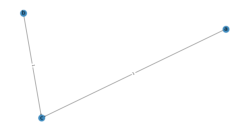
BNLearn is a Python library for bayesian learning. We can perform structure learning very easily:
import bnlearn as bn

model = bn.structure_learning.fit(data)
G = bn.plot(model)

which is precisely the model that we have designed.