Kernel Methods
Definition
A kernel $K(x,x’)$ is a function that obeys the property
\[K(x,x')=\langle\Phi(x)\cdot\Phi(x')\rangle\]where $\langle\cdot\rangle$ denotes inner product in some vector space $\mathbb{V}$ and $\Phi(x)$ is a mapping from $x\in \mathbb{R}^d$ to $\mathbb{V}$, known as feature map. Examples:
- Any polynomial function of $\langle x\cdot x’\rangle$ is a kernel. This is because of the property that
- Using this, we can also show that the gaussian function is a kernel:
Regression
In the KNN algorithm we take the K nearest neighbors of point $x$ and average their values. That is,
\[\hat{y}|_x=\frac{1}{K}\sum_{i\in \text{K-neighbors(x)}} y_i|_x\]We can put it differently by considering probabilities $p(y_i|x)=\frac{1}{K}$ and attach them to the $K$ neighbors of point $x$. Then the above average becomes
\[\hat{y}|_x=E(y|x)\]Rather than giving equal weights to the neighbors, we can give weights that decay with distance. This allows us to include contributions from very far without introducing additional bias. For example, using the gaussian function kernel we can write
\[p(y_i,x)=\frac{1}{N}\exp{\left(-\frac{|x-x_i|^2}{d^2}\right)}\]where $N$ is the number of datapoints in the training set and $d$ is the Kernel width. It follows that
\[p(y_i|x)=\frac{p(y_i,x)}{\sum_i p(y_i,x)}\]and
\[E(y|x)=\frac{\sum_i y_ip(y_i,x)}{\sum_i p(y_i,x)}\]Note that for $d\rightarrow \infty$ all the data-points contribute equally and $p(y_i|x)\rightarrow\frac{1}{N}$. This is the limiting case of KNN algorithm when we include all the neighbors. We have seen that when the number of neighbors is large variance decreases but bias increases. However, for $d$ small, only the closest neighbors contribute. In this case we expecte variance to increase, but bias to be small.
As an example, we generate an artificial training dataset for the line:
\[f(x)=x^2 e^{-0.05x}\]and fit a gaussian kernel.
def f(x):
    y=x*x*np.exp(-0.05*x)
    return y

xtrain=np.arange(0,200)
eps=np.random.normal(0,10,200)
y=f(x)
ytrain=y+eps

class KernelRg:
    def __init__(self,d):
        self.d=d

    def fit(self,x,y):
        self.x=x
        self.y=y

    def predict(self,x):
        z=x.reshape(-1,1)
        mu=self.x.reshape(1,-1)
        r=self.f(z-mu)
        r_=r*(self.y.reshape(1,-1))
        r_=r_.sum(1)
        N=r.sum(1)
        return r_/N

    def prob(self,x):
        z=x.reshape(-1,1)
        mu=self.x.reshape(1,-1)
        r=self.f(z-mu)
        p=r.sum(1)

        return p

    def le(self,x):
        p=self.prob(x)
        L=-np.log(p).sum()

        return L

    def f(self,x):
        p=1/np.sqrt(2*np.pi*self.d**2)*np.exp(-(x)*(x)/(2*self.d**2))

        return p

K=KernelRg(d=0.1)
K.fit(xtrain,ytrain)

sample=np.arange(0,200,0.2)
ysample=K.predict(sample)
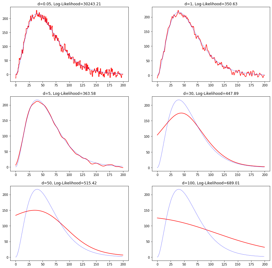
We plot a prediction for various widths $d$ including the log-likelihood defined as
\[\text{Log-Likelihood}=-\sum_x \ln(\sum_i p(y_i,x))\]
For small $d$ we see a lot of variance and for larger values of $d$ the function changes very slowly. In fact, when $d$ is small the contributions from the nearest neighbors contribute more strongly and as such variance increases. But for large $d$ all the data-points start contributing equally which increases bias.
Density Estimation
One way to estimate a density distribution is to build a histogram. In a histogram we partition the feature space in buckets and then count how many data-points fall in those buckets. However, the histogram depends on a partition choice, so it is not unique, and does not provide a smooth, continuous distribution function.
A way to resolve these issues is by considering the empirical distribution. It can be represented as a sum of Dirac delta functions:
\[f(x)=\frac{1}{N}\sum_{x_i} \delta(x-x_i)\]where $N$ is the number of datapoints $x_i$. In contrast with the histogram, this distribution is unique and can be used to calculate the probability for any $x$. For example, the probability of finding $x$ in the interval $[a,b]$ is given by
\[\int_a^bf(x)dx=\frac{1}{N}\sum_{x_i} \int_a^b\delta(x-x_i)dx=\frac{\# x_i\in[a,b]}{N}\]Despite providing an accurate representation of the sample distribution, $f(x)$ is highly singular and cannot be used in practice. Instead we can consider an approximation, which is smooth, by using the identity:
\[\delta(x-x')=\lim_{d\rightarrow 0}\frac{1}{\sqrt{2\pi}d}e^{-(x-x')^2/2d^2}\]We can approximate the sum of delta functions using a finite $d$, that is,
\[f(x)\simeq \frac{1}{N}\sum_{x_i}\frac{1}{\sqrt{2\pi}d}e^{-(x-x_i)^2/2d^2}\]which reproduces exactly $f(x)$ in the limit $d\rightarrow 0$. Here $d$, the width, acts as a regulator of the singular behaviour of the Dirac delta function.
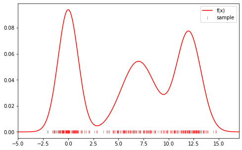
As an example, we sample a set of $x_i$ from the distribution:
\[f(x)=\frac{1}{3\sqrt{2\pi 2}}e^{-x^2/4}+\frac{1}{3\sqrt{2\pi 6}}e^{-(x-7)^2/6}+\frac{1}{3\sqrt{2\pi 3}}e^{-(x-12)^2/3}\]
Then we fit the training set with a gaussian Kernel:
class KernelDensity:
    def __init__(self,d):
        self.d=d

    def fit(self,xtrain):
        self.xtrain=xtrain
        self.n=xtrain.shape[0]

    def predict(self,x):
        z=x.reshape(-1,1)
        mu=self.xtrain.reshape(1,-1)
        r=self.f(z-mu).sum(1)

        return r/self.n

    def le(self,x):
        r=self.predict(x)
        r=-np.log(r).sum()

        return r

    def f(self,x):
        p=1/np.sqrt(2*np.pi*self.d**2)*np.exp(-(x)*(x)/(2*self.d**2))

        return p

K=KernelDensity(1)
K.fit(xtrain)
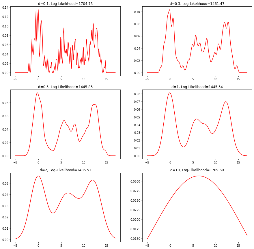
This is the estimated density for various values of $d$ including the corresponding log-likelihood:

Classification
In classification, we have a set $(x_i,c_i)$ with $c_i=0,1,\ldots$ the labels. We are interested in estimating
\[P(c|x)\]from the data. This can be written as
\[P(c|x)=\frac{P(x|c)P(c)}{\sum_{c'} P(x|c')P(c')}\]So using the previous results on density estimation, we can calculate
\[P(x|c)\]for each class using a kernel. The probability $P(c)$ is easily estimated using the maximum-likelihood principle, giving
\[P(c)=\frac{\# (c_i=c)}{N}\]with $N$ the number of data-points.
Example in Python
from sklearn.datasets import load_breast_cancer
from sklearn.model_selection import train_test_split
from sklearn.preprocessing import StandardScaler

data=load_breast_cancer()
X=data['data']
Y=data['target']
We use StandardScaler to standardize the dataset:
ss=StandardScaler()
X_s=ss.fit_transform(X)

xtrain,xtest,ytrain,ytest=train_test_split(X_s,Y,test_size=0.2)
Then we define the Kernel model:
class KernelClf:
    def __init__(self,d):
        self.d=d

    def fit(self,x,y):
        labels, counts=np.unique(Y, return_counts=True)
        N=counts.sum()
        self.pc={l: c/N for l,c in zip(labels, counts)}

        self.kernels={}
        for l in labels:
            id_c= y==l
            x_c= x[id_c]
            K=Kernel(self.d)
            K.fit(x_c)
            self.kernels[l]=K

    def predict_prob(self,x):
        pv=[K.predict(x)*self.pc[c] for c,K in self.kernels.items()]
        P=sum(pv)
        prob=[p/P for p in pv]
        prob=np.concatenate([p.reshape(-1,1) for p in prob],axis=1)

        return prob

    def predict(self,x):
        pv=[K.predict(x)*self.pc[c] for c,K in self.kernels.items()]
        P=sum(pv)
        prob=[p/P for p in pv]
        prob=np.concatenate([p.reshape(-1,1) for p in prob],axis=1)

        return prob.argmax(1)
Train:
Kclf=KernelClf(d=0.5)
Kclf.fit(xtrain,ytrain)

ypred=Kclf.predict(xtest)
acc=(ypred==ytest).mean()
97.37%