Power Test
Statistical Power
The power statistic is defined as the probability
\[\text{power}=P(\text{reject }H_0|H_1\text{ True})\]where $H_0$ is the null hypothesis and $H_1$ is the alternative hypothesis.
We can model the t-statistics of both hypothesis using the Student’s t-distribution.

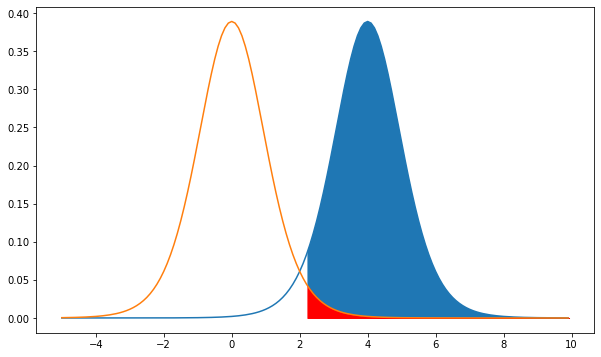
On the right is the distribution for the $H_1$ hypothesis while on the left we have the $H_0$ or null hypothesis. The area in red is the probability of rejecting the null hypothesis given that $H_0$ is true. This is the significance level that is usually is set to 5%. The area in blue is the probability of rejecting the null given that $H_1$ is true. If the distributions are far apart then the power approaches 1, while if they are close to each other the power is small.
Consider a statistical test for the difference of means of two samples with equal sizes $n_1=n_2=n$ and variance. The t-statistic is
\[t=\frac{\bar{X}_1-\bar{X}_2}{s_p\sqrt{\frac{2}{n}}}\]where $s_p$ is the pooled variance:
\[s_p^2=\frac{s_1^2+s_2^2}{2}\]and $\text{df}=2n-2$ are the number of degrees of freedom.
For large $n$ the Student t-distribution approaches a standard normal distribution. So we can calculate the power as
\[\text{power}=\int_{t_{\alpha}}^{\infty}dt\frac{e^{-(t-t^*)^2/2}}{\sqrt{2\pi}}=1-\Phi(t_{\alpha}-t^*)\]Here $t_{\alpha}$ is the value for which the null hypothesis is rejected, and $t^*$ is the expected value when $H_1$ is true.
The value of power is usually set at 80%, which means that $\Phi(t_{\alpha}-t^*)=0.2$ or:
\[t^*-t_{\alpha}\simeq 0.842\]while $t_{\alpha}\simeq 1.96$, which is the value for which $\Phi(t_{\alpha})=0.975$. Definining the effect size as:
\[d=\frac{\bar{X}_1-\bar{X}_2}{s_p}\]we can calculate the sample size with
\[n=2(1.96+0.842)^2/d^2\]