Probably Approximately Correct (PAC)

Table of Contents

1. The learning problem
2. Finite hypothesis classes are PAC learnable
3. Agnostic learning

1. The learning problem

PAC stands for “probably approximately correct”. In machine learning we want to find a hypothesis that is as close as possible to the ground truth. Since we only have access to a sample of the real distribution, the hypothesis that one builds is itself a function of the sample data, and therefore it is a random variable. The problem that we want to solve is whether the sample error incurred in choosing a particular hypothesis is approximately the same as the exact distribution error, within a certain confidence interval.

Suppose we have a binary classification problem (the same applies for multi-class) with classes $y_i\in \{y_0,y_1\}$, and we are given a training dataset $S$ with $m$ data-points. Each data-point is characterised by $Q$ features, and represented as a vector $q=(q_1,q_2,\ldots,q_Q)$. We want to find a map $\mathcal{f}$ between these features and the corresponding class $y$:

$$\mathcal{f}: (q_1,q_2,\ldots,q_Q)\rightarrow \{y_0,y_1\}$$

This map, however, does not always exist. There are problems for which we can only determine the class up to a certain confidence level. In this case we say that the learning problem is agnostic, while when the map exists we say that the problem is realisable. For example, image recognition is an agnostic problem.

Let us assume for the moment that such a map exists, that is, we are in the realisable case. The learner chooses a set of hypothesis $\mathcal{H}={h_1,\ldots,h_n}$ and by doing this it introduces bias in the problem- a different learner may chose a different set of hypothesis. Then, in order to find the hypothesis that most accurately represents the data, the learner chooses one that has the smallest empirical risk, that is the error on the training set. In other words, one tries to find the minimum of the sample loss function

$$L_S(h)=\frac{1}{m}\sum_{i=1:m}\mathbb{1}\left[h(x_i)\neq y(x_i)\right],\;h\in \mathcal{H}$$

with $\mathbb{1}(.)$ the Kronecker delta function. Denote the solution of this optimisation problem as $h_S$. The true or generalization error is defined instead as the unbiased average

$$L(D,h)=\sum_x\mathbb{1}\left[h(x)\neq y(x)\right]D(x)$$

where $D(x)$ is the real distribution. In the case of classification, the generalisation error is also the probability of misclassifying a point

$$L(D,h)=\mathbb{P}_{x\sim D(x)}(h(x)\neq y(x))$$

If we choose appropriately $\mathcal{H}$ we may find $\text{min}\;L_S(h_S)=0$. This can happen, for example, by memorising the data. In this case, we say that the hypothesis is overfitting the data. Although memorising the data results in zero empirical error, the solution is not very instructive because it does not give information of how well it will perform on unseen data.

The overfitting solution performs very well on the data because the learner used prior knowledge to choose a hypothesis set with sufficient capacity (or complexity) to accommodate the entire dataset. In the above minimisation problem, one should find a solution that does well (small error) on a large number of samples rather then having a very small error in the given sample. Overfitting solutions should be avoided as they can lead to misleading conclusions. Instead, the learner should aim at obtaining a training error that is comparable to the error obtained with different samples.

To make things practical, consider the problem of classifying points on a 2D plane as red or blue. The decision boundary is a circumference of radius $R$ concentric with the origin of the plane, which colours points that are inside as red and outside as blue. See figure below. The training dataset consists of $m$ data-points $\mathbb{x}=(x_1,x_2)$ sampled independently and identically distributed (i.i.d) from a distribution $D(x)$.

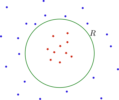
Here the circumference $R$ denotes the ground truth which classifies points as red or blue, depending on whether they are inside or outside of the circle, respectively.

The learning problem is to find a hypothesis $h(x): x\rightarrow y={\text{blue},\text{red}}$ that has small error on unseen data.

Assuming that the learner has prior knowledge of the ground truth (realisability assumption), that is, the learner assumes that the best hypothesis is a circumference but it does not how its radius. One of the simplest algorithms is to consider the set of concentric circumferences and minimise the empirical risk. This can be achieved by drawing a decision boundary that is as close as possible to the most outward red (or inward blue data-points). This guarantees that when the sample has infinite number of points, that is $m\rightarrow \infty$, we recover the exact decision boundary: the circumference $R$. The empirical risk minimisation problem gives the solution represented in the figure below by the circumference $R’$. However, newly generated data-points may lie in between $R’$ and $R$, and therefore would be misclassified.

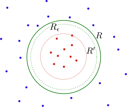
a) The hypothesis $h$ is a circumference of radius $R’$ concentric with the origin and it is determined by the most outward red data-point. This ensures that all training set $S$ is correctly classified. b) The circumference of radius $R_{\epsilon}$ corresponds to a hypothesis $h_{\epsilon}$ that has generalization error $L(D,h_{\epsilon})=\epsilon$.

Given that this is an overfitting solution, one has to be careful of how well it generalises. It is possible that the generalisation error is small for such a solution, but one has to be confident of how common this situation may be. If the sample that led to that solution is a rare event then we should not trust its predictions, and we should expect large generalization error. Therefore we are interested in bounding the probability of making a bad prediction, that is,

$$\mathbb{P}_{S \sim D^m(x)}(L(D,h_S)>\epsilon)<\delta \tag{1}$$

Conversely, this tells us with confidence of at least $1-\delta$ that

$$L(D,h_S)\leq\epsilon\tag{2}$$

A PAC learnable hypothesis is a hypothesis for which one can put a bound on the probability of the form Eq.1 with $\epsilon, \delta$ arbitrary.

In the case of the circumference example, define $R_{\epsilon}$ for which $L(D,h_{\epsilon})=\epsilon$, with $h_{\epsilon}$ the corresponding solution. Any hypothesis corresponding to a radius less than $R_{\epsilon}$ leads to a generalisation error larger than $\epsilon$. The probability of sampling a point and falling in the region between $R_{\epsilon}$ and $R$ is precisely $\epsilon$. Conversely the probability of falling outside that region is $1-\epsilon$. It is then easy to see that the probability that we need equals

$$\mathbb{P}_{S \sim D^m(x)}(L(D,h_S)>\epsilon)=(1-\epsilon)^m$$

Using the bound $1-\epsilon<e^{-\epsilon}$ we can choose $\delta=e^{-\epsilon m}$, and thus equivalently $\epsilon=\frac{1}{m}\ln\left(\frac{1}{\delta}\right)$. Hence using equation \eqref{eq2}, we have

$$L(D,h_S)\leq\frac{1}{m}\ln\left(\frac{1}{\delta}\right)$$

with probability $1-\delta$.

2. Finite hypothesis classes are PAC learnable

Let us assume that we have a finite hypothesis class with $N$ hypothesis, that is, $\mathcal{H}_N={h_1,\ldots,h_N}$, and that this class is realisable, meaning that it contains a $h^\star$ for which $L_S(h^\star)=0\;\forall S$. We want to upper bound the generalisation error of a hypothesis $h_S$ obtained using empirical risk minimisation, that is, we want to find a bound of the form

\[\mathbb{P}_{x\sim D(x)}(S: L(D,h_S)>\epsilon)<\delta\tag{3}\label{eq3}\]

Define $\mathcal{H}_B$ as the set of hypotheses that have generalisation error larger than $\epsilon$ (it does not necessarily minimise the emprirical risk). We call this the set of bad hypotheses

$$\mathcal{H}_B=\{h\in \mathcal{H}_N: L(D,h)>\epsilon\}$$

Similarly one can define the set of misleading training sets, as those that lead to a hypothesis $h_S\in \mathcal{H}_B$ with $L_S(h_S)=0$. That is,

$$M=\{S: h\exists \mathcal{H}_B, L_S(h)=0\}$$

Since we assume the class is realisable, the hypothesis $h_S$ in equation Eq.3 must have $L_S(h_S)=0$, and therefore the sample data is a misleading dataset. So we need the probability of sampling a misleading dataset $S\in M$. Using

$$\begin{align} M=\cup_{h\in \mathcal{H}_B} \{S: L_S(h)=0\} \end{align}$$

and the property $\mathbb{P}(A\cup B)<\mathbb{P}(A)+\mathbb{P}(B)$, we have

$$\begin{align} \mathbb{P}(S\in M)\leq \sum_{h\in \mathcal{H}_B} \mathbb{P}(S: L_S(h)=0) \end{align}$$

Now for each $h\in\mathcal{H}$ we can put a bound on $\mathbb{P}(S: L_S(h)=0)$. Since we want $L(D,h)>\epsilon$, the probability of misclassifying a data-point is larger than $\epsilon$, and conversely a point will correctly classified with probability $1-\leq \epsilon$. Therefore, as the solution is always overfitting and so all the points are correctly classified, we have

$$\mathbb{P}(S: L_S(h)=0)\leq (1-\epsilon)^m$$

The final bound becomes

$$\begin{align} \mathbb{P}(S\in M)\leq \sum_{h\in \mathcal{H}_B}(1-\epsilon)^m\leq |\mathcal{H}|(1-\epsilon)^m\leq |\mathcal{H}|e^{-\epsilon m} \end{align}$$

Setting $\delta=\mid\mathcal{H}\mid e^{-\epsilon m}$, we have with a probability of at least $1-\delta$ that

$$L(D,h_S)\leq \frac{1}{m}\ln\left(\frac{\mid\mathcal{H}\mid}{\delta}\right)$$

3. Agnostic learning

In agnostic learning we do not have anymore an exact mapping between the features and the classes. Instead the classes themselves are sampled from a probability distribution given the features, that is, we have $P(y|x)$. In the realisable example this probability is always $P(y|x)=0,1$. Given this we extend the distribution to both the features and the classes so we have $D(x,y)$.

The definition of generalisation error is slightly changed to $L(D,h)=\sum_{x,y}\mathbb{1}(h(x)\neq y)D(x,y)$

Because we do not have anymore the realisability condition, showing that a problem is PAC learnable is a bit more complicated. For this purpose we use one of the most useful inequalities in statistics:

Hoeffding’s Inequality: $\mathbb{P}(|\bar{x}-\langle x\rangle|>\epsilon)\leq 2e^{-2 m\epsilon^2/(b-a)^2}$

for a random variable $x$ and any distribution. Here $\bar{x}$ is the sample mean, $\langle x \rangle$ is the distribution average and $a\leq x\leq b$. We can apply this property to the empirical loss and the generalisation loss. Since they are quantities between zero and one (they are probabilities), we have

$$\mathbb{P}(|L_S(h)-L(D,h)|>\epsilon)\leq 2e^{-2 m\epsilon^2}$$

We are interested in the probability of sampling a training set which gives a misleading prediction. So we want

$$\mathbb{P}_{S\sim D^m}(h\exists \mathcal{H}, |L_S(h)-L(D,h)|>\epsilon)\leq \sum_{h\in \mathcal{H}} \mathbb{P}_{S\sim D^m}(|L_S(h)-L(D,h)|>\epsilon)$$

and thus using Hoeffding’s inequality we have $\mathbb{P}_{S\sim D^m}(h\exists \mathcal{H}, |L_S(h)-L(D,h)|>\epsilon)\leq \mid\mathcal{H}\mid 2e^{-2\epsilon^2m}$ We set $\delta=2\mid\mathcal{H}\mid e^{-2 m\epsilon^2}$, and conclude

$$|L_S(h)-L(D,h)|\leq \sqrt{\frac{1}{2m}\ln\left(\frac{2\mid\mathcal{H}\mid}{\delta}\right)},\;\forall h\in \mathcal{H}$$

Say that we have $L(D,h)>L_S(h)$ for $h=h_S$, the solution we obtain after minimising the empirical loss, then

$$L(D,h)\leq L_S(h)+\sqrt{\frac{1}{2m}\ln\left(\frac{2\mid\mathcal{H}\mid}{\delta}\right)}\tag{4}$$

This equation demonstrates clearly the trouble with overfitting. To memorise the data we need to use hypothesis classes with large dimension, so the solution has enough capacity to accommodate each data-point. This makes the second term on r.h.s of the inequality Eq.4 very large, loosening the bound on the generalisation error instead of making it tighter. The fact is that we should minimise the empirical error together with that term, so we make the bound on the true error smaller. This leads us to the idea of regularisation in machine learning, whereby the empirical loss is endowed with correction terms that mitigate highly complex solutions.

References

[1] Understanding Machine Learning: from Theory to Algorithms, Shai Ben-David and Shai Shalev-Shwartz