Bayes Optimal Classifier

Optimal classifier
Multiple classes

1. Optimal classifier

The Bayes optimal classifier is a binary predictor which has the lowest generalisation error. That is, for any other predictor $g$ we always have

\[L(D,h_{\text{Bayes}})\leq L(D,g)\]

The Bayes predictor is defined as follows:

\[h_{\text{Bayes}}=\text{argmax}_{y}P(y|x)\]

Proof: Define $L(D,g)=\sum_{x}\mathbb{1}\left[g(x)\neq y(x)\right]D(x,y)$. Then use the Bayes property $D(x,y)=D(y|x)D(x)$ and the fact that we have only two classes, say $y=0,1$:

\[L(D,g)=\sum_{x:g(x)=0}D(y=1|x)D(x)+\sum_{x:g(x)=1}D(y=0|x)D(x)\]

Use the property that $a\geq \text{Min}(a,b)$ and write

\[\begin{equation}\begin{split}L(D,g)\geq\sum_{x:g(x)=0}\text{Min}\big(D(y=1|x),D(y=0|x)\big)D(x)+\\ \sum_{x:g(x)=1}\text{Min}\big(D(y=1|x),D(y=0|x)\big)D(x)\\ =\sum_{x}\text{Min}\big(D(y=1|x),D(y=0|x)\big)D(x)\end{split}\end{equation}\]

Note that the r.h.s is precisely the loss of the Bayes classifier. That is,

\[\begin{equation}\begin{split}L(D,h_{\text{Bayes}})=&\sum_{x:h(x)=0}D(y=1|x)D(x)+\sum_{x:h(x)=1}D(y=0|x)D(x)\\ =&\sum_{D(y=1|x)<D(y=0|x)}D(y=1|x)D(x)+\sum_{D(y=1|x)>D(y=0|x)}D(y=0|x)D(x)\end{split}\end{equation}\]

2. Multiple classes

Can we generalise this to multi-classes? We can use $a\geq \text{Min}(a,b,c,\ldots)$ to write

\[\begin{equation} \begin{split} L(D,g)\geq &\sum_{x:g(x)\neq y_1}\text{Min}\big(D(y_1|x),D(y_2|x),\ldots\big)D(x)+\\ &\sum_{x:g(x)\neq y_2}\text{Min}\big(D(y_1|x),D(y_2|x),\ldots\big)D(x)+\ldots \end{split} \end{equation}\]

Suppose we extend the Bayes optimal classifier to more classes by predicting the class that has higher probability. Then we have

\[\begin{equation}\begin{split} L(D,h)=\sum_{x:h(x)=y_1\cup h(x)=y_2\ldots}D(y_0|x)D(x)+\sum_{x:h(x)=y_0\cup h(x)=y_2\ldots}D(y_1|x)D(x)+\ldots \end{split}\end{equation}\]

Since $h(x)$ is a predictor the sets $S_i=\{x:h(x)=y_i\}$ are disjoint and so we can simplify the sums above. For example

\[\begin{equation}\begin{split}\sum_{x:h(x)=y_1\cup h(x)=y_2\ldots}D(y_0|x)D(x)=\sum_{x:h(x)=y_1}D(y_0|x)D(x)+\sum_{x:h(x)=y_2\ldots}D(y_0|x)D(x)+\ldots\end{split}\end{equation}\]

The issue we face now is that since we have multiple classes the maximum value does not determine uniquely the minimum value, and vice-versa, and hence we cannot apply the reasoning used in the binary case. Following similar steps as before, one can show that the multi-class Bayes classifier does not saturate the bound Eq.1. As a matter of fact there is no classifier that saturates the bound Eq.1. For that to happen we would need a classifier $h(x)$ such that when $h(x)=y_i$ we have $\text{Min}\big(D(y_1|x),D(y_2|x),\ldots\big)=D(y_{k\neq i}|x)\,\forall i,k$. This means that for a fixed $i$ we have $D(y_{k\neq i}|x)=D(y_{j\neq i}|x)\, \forall k,j\neq i$. It is then easy to see that this implies that $D(y_i|x)$ is a constant, independent of $x$, contradicting our assumption.

Python implementation

import numpy as np
import pandas as pd
import matplotlib.pyplot as plt
import seaborn as sns

from sklearn.naive_bayes import GaussianNB

We compare three different hypotheses:

Optimal Bayes: $h_{\text{Bayes}}$
Circumference hypothesis: $h$
Gaussian Naive Bayes: $h_{GNB}$

#P(y|x) definition
def prob(x,p=0.7,q=0.3): #prob of y=1

    if x[0]**2+x[1]**2>=1:
        return p
    else:
        return q

#coloring function
def color(p):

    if np.random.rand()<=prob(p):
        return 'blue' #y=1
    else:
        return 'red' #y=0

The code that defines the various hypotheses:

def h(x,r=1.2):
    if x[0]**2+x[1]**2>=r: #if r=1 then h(x)=bayes(x)
        return 'blue'
    else:
        return 'red'

def bayes(x):
    if prob(x)>=0.5:
        return 'blue'
    else:
        return 'red'

def GNB(df):
    model=GaussianNB()
    model.fit(df[['x','y']],df['sample'])
    ypred=model.predict(df[['x','y']])

    return ypred

errors=[]
for i in range(10): #draw multiple samples from multivariate_normal
    sample= np.random.multivariate_normal([0,0],[[1,0],[0,1]],1000)
    class_y=[color(p) for p in sample]
    df=pd.DataFrame(sample, columns=["x","y"])
    df['sample']=pd.Series(class_y)
    df['h_bayes']=df[['x','y']].apply(bayes,1)
    df['h']=df[['x','y']].apply(h,1)
    df['GNB']=GNB(df)

    error_GNB=(df['sample']!=df['GNB']).astype(int).mean()
    error_bayes=(df['sample']!=df['h_bayes']).astype(int).mean()
    error_h=(df['sample']!=df['h']).astype(int).mean()

    errors.append([error_h,error_GNB,error_bayes])

then check whether the other hypotheses have smaller error:

len([e for e in errors if e[0]<e[2] or e[1]<e[2]])

Note that these are the sample errors. Therefore, it is possible to find an error smaller than the Bayes error. However, if we take large samples it becomes almost improbable for that to happen.

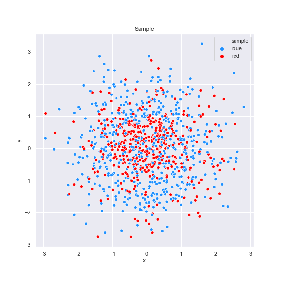
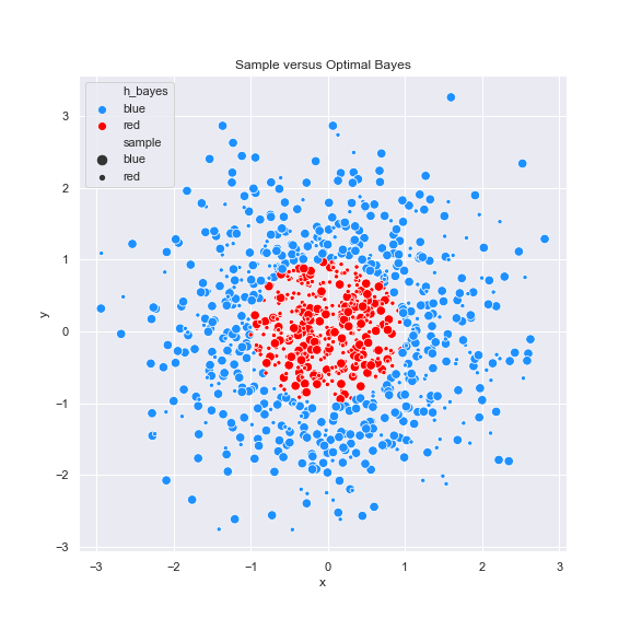
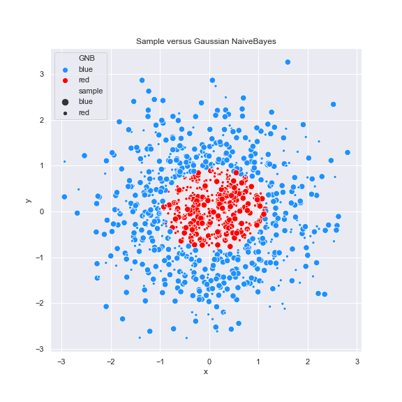
Some plots:

References

[1] Understanding Machine Learning: from Theory to Algorithms, Shai Ben-David and Shai Shalev-Shwartz

Table of contents

1. Optimal classifier

2. Multiple classes

Python implementation

References