VC dimension
Table of contents
1. VC dimension
VC stands for Vapnik-Chervonenkis. The VC dimension plays the role of $\mathcal{H}$, when $\mathcal{H}$ has an infinite number of hypotheses. In the post on “PAC learning” we have shown that the circumference hypothesis is PAC learnable despite the class being infinite. One can find several other examples that depend on continuous parameters, but they are nevertheless learnable. In this post, we analyze necessary conditions for infinite-dimensional classes to be PAC learnable.
To do this, first we need to understand the concept of shattering. Say we have a set of hypotheses $\mathcal{H}={h_a(x)}$ from a domain $\chi$ to ${0,1}$. Here $a$ is(are) a continuous parameter(s). Consider a subset $C\subset \chi$ consisting of a number of points $C={c_1,c_2,\ldots,c_n}$. The restriction of a hypothesis $h_a(x)\in\mathcal{H}$ to $C$ is ${h_a(c_1),h_a(c_2),\dots,h_a(c_n)}$. By dialling the continuous parameter $a$ we generate images of the restriction $(h_a(c_1),h_a(c_2),\dots,h_a(c_n))=(1,0,1,\ldots),(0,0,1,\ldots),\ldots$. Depending on the set $C$ we may or not generate all the possible images, which total to $2^n$. When it generates all possible images we say that $\mathcal{H}$ shatters $C$. The VC dimension is the dimension of the largest set $C$ that can be shattered.
Examples:
1) Set of thresholds
\[h_a(x)=\mathbb{1}_{x\geq a}\]which returns $1$ for $x\geq a$ and $0$ otherwise. Clearly for any $c_1$, $h_a(c_1)$ spans ${0,1}$. However, if we have an additional point $c_2>c_1$ then we cannot generate the image $(h(c_1),h(c_2))=(1,0)$. In fact generalising for arbitrary number of points with $c_1<c_2<\ldots<c_n$ we always have that if $h_(c_1)=1$ then all the reamining images are $h(c_2),\ldots,h(c_n)=1$. Therefore the VC dimension is
\[VC_{\text{dim}}=1\]Note that this the same set of hypothesis in the cirumference case (see post “PAC learning”).
2) Set of intervals
\[h_{a,b}(x)=\mathbb{1}_{a\leq x\leq b}\], which returns one for a point inside the interval $[a,b]$ and zero otherwise. Clearly $h_{a,b}$ shatters a single point. We can easily see that two points can also be shattered. However, a set with three points cannot be shattered. In the case we have $h_{a,b}(c_1)=1$ and $h_{a,b}(c_2)=0$ with $c_2>c_1$ a third point $c_3>c_2$ cannot have $h_{a,b}(c_3)=1$. Therefore the VC dimension is $VC_{\text{dim}}=2$.
3) Set of hyperplanes in $\mathbb{R}^2$.
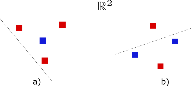
The hyperplane divides the space into two regions. A point falling on one side will have class zero, while if it falls on the other, it will have class one. The same hyperplane can give rise to two different hypotheses by interchanging the labels between the sides. It is easy to see that we can shatter a two-point set. Consider now a three-point set. If they are collinear, then there are always two combinations $(1,0,1)$ and $(0,1,0)$ that cannot be shattered. If they are not collinear, then we can generate the dichotomies with two ones and one zero, like $(1,1,0)$, and two zeros and one, such as $(0,0,1)$. The remaining dichotomies $(0,0,0)$ and $(1,1,1)$ are generated by interchanging the sides. Therefore we can shatter the set of three non-collinear points. Consider now a set of four points and assume that three are non-collinear (if they are collinear, then we fall back in the previous situation). The dichotomies depicted in Fig.1 show two examples that are not possible. Thus showing that there is no four-point set that can be shattered. The VC dimension is therefore
\[VC_{\text{dim}}=3\]4) Hyperplanes in $\mathbb{R}^d$.
One can show that the VC dimension is
\[VC_{\text{dim}}=d+1\]The demonstration can be found in the post “Hyperplanes and classification”. This will be very useful when studying support-vector-machines.

Fig.1 Dichotomies that cannot be realised. a) The fourth point is in the interior of the triangle. b) The set forms a convex four-polygon.
The VC dimension provides a measure of how complex a hypothesis class can be. If the class is increasingly complex, it allows for larger sets to be shattered. This measure is purely combinatorial and does not rely on which the distribution of the points.
2. The growth function
The growth function counts how many ways we can classify a fixed size set using a hypothesis class. The proper definition is
When the set $x_1,\ldots,x_m$ is shattered by $\mathcal{H}$ one has $\Pi(m)=2^m$. If in addition this is the largest shattered set, then $\Pi(m)=2^{VC_{\text{dim}}}$.
One of the most critical aspects of the growth function is that for $m>VC_{\text{dim}}$, $\Pi(m)$ always has polynomial growth rather than exponential. This is demonstrated using the following statement:
Sauer’s Lemma:
Let $VC_{\text{dim}}=d$. Then for all $m$
\[\Pi(m)\leq \sum_{i=0}^{d}\left(\begin{array}{c}m \\ i\end{array}\right)\]For $t\leq m$ we have
\[\sum_{i=0}^{d}\left(\begin{array}{c}m \\ i\end{array}\right)\leq \sum_{i=0}^{m}\left(\begin{array}{c}m \\ i\end{array}\right)\left(\frac{m}{t}\right)^{d-i}=\left(\frac{m}{t}\right)^d\left(1+\frac{t}{m}\right)^m\]Using that $1+x\leq e^x, \forall x$, we get
\[\left(\frac{m}{t}\right)^d\left(1+\frac{t}{m}\right)^m\leq \left(\frac{m}{t}\right)^d e^t\]Now we can set $t=d$ for which the bound becomes optimal, that is, $t^{-d} e^t\geq d^{-d}e^d$ (we can do this by finding the minimum of $t-d\ln(t)$). Hence we obtain
\[\Pi(m)\leq \left(\frac{m}{d}\right)^d e^d\]3. The generalisation bound for infinite classes
The Vapnik-Chervonenkis theorem (1971) states that, for any $\epsilon$,
We can now understand the importance of the VC dimension. We have learnt that if VC dimension is finite than the growth function $\Pi(m)$ grows polynomially for $m>VC_{\text{dim}}$. This implies from the inequality Eq.3 that
\[m\rightarrow \infty,\;|L_S(h)-L_D(h)|\rightarrow 0,\;\text{in propability}\]This means that we can find arbitrary $\epsilon$ and $\delta$ such that for $m\geq m_{\mathcal{H}}$, the sample complexity, the problem is PAC learnable.
References
[1] Understanding Machine Learning: from Theory to Algorithms, Shai Ben-David and Shai Shalev-Shwartz
[2] A probabilistic theory of pattern recognition, Luc Devroye, Laszlo Gyorfi, Gabor Lugosi
[3] Foundations of machine learning, M. Mohri, A. Rostamizadeh, A. Talwalkar