Bias-Variance/Complexity tradeoff
1. Basic concept
Let $h_S$ be the solution of an ERM algorithm. We decompose the generalization error as
\[L_D(h_S)=\epsilon_{app}+\epsilon_{est}\]with
\[\epsilon_{app}=\text{min}_{h\in \mathcal{H}}L_D(h),\;\;\epsilon_{est}=L_D(h_S)-\text{min}_{h\in \mathcal{H}}L_D(h)\]Here $\epsilon_{app}$ is the approximation error which is the smallest error one can achieve using the hypothesis class $\mathcal{H}$. This error is independent of the data and depends only on the choice of the hypothesis class. On the other hand, $\epsilon_{est}$ is the estimation error, that is, it measures how far the generalization error is from the approximation error. Since $h_S$ depends on the training set, the estimation error depends strongly on the training data.
To reduce the approximation error we need a more complex hypothesis class but this might make the estimation error worse, since a more complex hypothesis may lead to overfitting. On the other hand, a smaller hypothesis class, that is, less complex, reduces the estimation error, because $h_S$ and $\text{argmin}_hL_D(h)$ are now closer, but it increases the approximation error because of underfitting. This tradeoff is known as the bias-complexity tradeoff.
Lets see how this works in practice. We create artificial data of around 1 million samples in a 10 dimensional feature space, according to the classification rule:
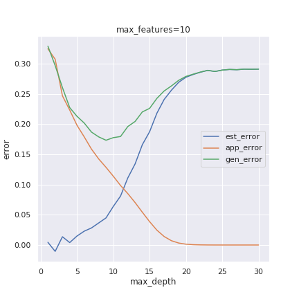
\[y(x)=\text{sign}(w^0_1\tanh(w^1_ix^i)+w^0_2\tanh(w^2_ix^i))\]where $w^1,w^2$ are 10 dimensional parameters and $(w^0_1,w^0_2)$ is a two parameter. For the classification we use a decision tree and adjust its max depth and number of features used in order to obtain different levels of complexity. Below we show the behaviour of the estimation (est_error), approximation (app_error) and generalization errors (gen_error):

To determine the approximation error, we train the decision tree on the full data while keeping fixed the number of features used and adjusting the tree’s depth (max_depth in the picture above). On the other hand, to determine the estimation error, we train the decision tree on 10% of the data (around 100k samples) for various depths and number of features. The generalization error is calculated on the remaining 90% of the data.
The generalization error curves show a tradeoff between bias and complexity. When the depth is smaller, so bias is more considerable, the approximation error grows, but the estimation error is smaller. In contrast, if we increase the depth, the approximation error becomes smaller, but the estimation error grows due to overfitting. The “sweet spot” occurs for an intermediate value of the depth, where the generalization error is a minimum.
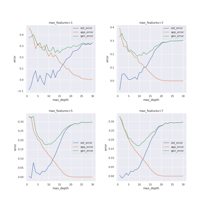
Similar behaviour is obtained for different number of features (max_features):

In the case of regression, we observe a similar tradeoff. Nevertheless, the analysis is slightly different. In general we want to model $y=f(x)+\epsilon$ where $\epsilon$ is noise with mean zero and standard deviation $\sigma$. So we use an algorithm to approximate $f(x)\simeq \hat{f}(x)$. Here $\hat{f}$ is the output of our algorithm.
The mean square error of a predictor (regression problem) can be decomposed as follows:
\[E_D[(y-\hat{f}(x_0;D))^2]=\text{Bias}^2+\text{Var}^2+\sigma^2\]where
\[\text{Bias}=E_D[\hat{f}(x_0;D)]-f(x_0)\]and
\[\text{Var}^2=E_D[E_D[\hat{f}(x_0;D)]-\hat{f}(x_0;D)]^2\]Note that the expectation $E_D$ is calculated by using different training datasets and $x_0$ is a reference point- the error will depend on this point which is kept fixed while averaging over different training sets.
We use fake data (1million samples) in a 10 dimensional feature space and target function
\[f(x)=(x.w)^4+(x.w)^2+x.h\]where $w,h$ are 10 dimensional parameter arrays. We use a decision tree regressor and adjust number of features used and max depth.

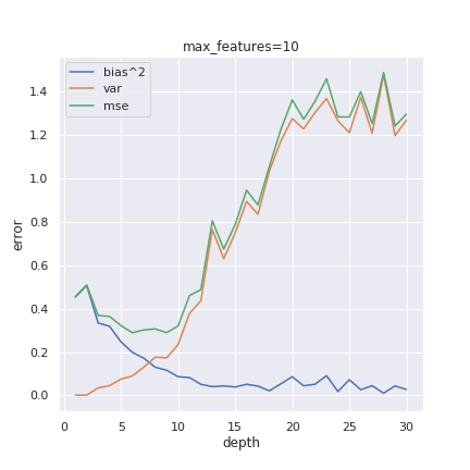
We sample about 20k data points in each iteration and fit the decision tree, calculate $\hat{f}(x_0)$ for a determined reference point and store this value. The bias is calculated from the mean of the difference $\hat{f}(x_0)-f(x_0)$ and for the variance, we compute $\hat{f}(x_0)$ after each training sample and then calculate the variance of that array.

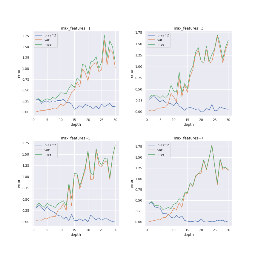
We can see that while variance increases with increasing depth, bias decreases. This behavior translates into a trade-off between bias and variance, explaining why the mean square error (mse) reachs its minimum at an intermediate depth.
2. Python implementation: Classification
Classification with Decision Tree:
import pandas as pd
import numpy as np
from sklearn.datasets import load_wine
from sklearn.model_selection import train_test_split
from sklearn.tree import DecisionTreeClassifier
from sklearn.metrics import accuracy_score
import progressbar
import multiprocessing as mp
Create artificial data
data=np.random.normal(0.1,3,(1000000,10))
w1=np.random.normal(1,5,10)
w2=np.random.normal(-1,10,10)
w0=np.random.normal(3,20,2)

y=w0[0]*np.tanh(data.dot(w1))+w0[1]*np.tanh(data.dot(w2))
y=np.sign(y)
Train and test data:
indices=np.arange(data.shape[0])
np.random.shuffle(indices)

l=int(0.1*len(indices)) #keep only 10% of the data
train_x=data[indices][:l]
test_x=data[indices][l:]
train_y=y[indices][:l]
test_y=y[indices][l:]

#add some noise to the training data
noise=np.random.normal(0,3,(l,10))
train_x=train_x+noise
Train the algorithm on the full dataset (1million). We can then determine the approximation error:
#Decision Tree parameters
params={'ccp_alpha': 0.0,
 'class_weight': None,
 'criterion': 'gini',
 'max_depth': 1,
 'max_features': 10,
 'max_leaf_nodes': None,
 'min_impurity_decrease': 0.0,
 'min_impurity_split': None,
 'min_samples_leaf': 1,
 'min_samples_split': 2,
 'min_weight_fraction_leaf': 0.0,
 'presort': 'deprecated',
 'random_state': None,
 'splitter': 'best'}

complexity={}
max_features=[1,3,5,7,10]

for max_f in progressbar.progressbar(max_features):
    params['max_features']=max_f
    complexity[max_f]=[]

    DT=DecisionTreeClassifier(**params)
    def pred(d):
        DT.max_depth=d
        DT.random_state=d
        DT.fit(data,y)
        acc=accuracy_score(DT.predict(data),y)
        return 1-acc

    #parallelize the calculation
    with mp.Pool(mp.cpu_count()) as pool:
        complexity[max_f]=pool.map(pred,[d for d in range(1,31)])
Now train on the train set:
max_features=[f for f in complexity]

learning={}
for f in max_features:
    params['max_features']=f
    learning[f]=[]
    for depth in progressbar.progressbar(range(1,31)):
        params['max_depth']=depth
        params['random_state']=depth+100
        DT=DecisionTreeClassifier(**params)
        DT.fit(train_x,train_y)
        acc=accuracy_score(DT.predict(test_x),test_y) #calculates the generalization error
        learning[f].append(1-acc)
3. Python implementation: Regression
Regression with Decision Tree:
import pandas as pd
import numpy as np
import progressbar
import matplotlib.pyplot as plt
import seaborn as sns
from sklearn.tree import DecisionTreeRegressor
from sklearn.metrics import mean_squared_error
import multiprocessing as mp
Data preparation
x=np.random.normal(0,1,(1000000,10))
w=np.random.normal(0,0.1,10)
h=np.random.normal(0,0.1,10)

#target function
def fnt(x):
    return (x.dot(w))**2+x.dot(h)+(x.dot(w))**4

y=fnt(x)+np.random.normal(0,1,y.shape[0])
Decision Tree regressor:
params={'criterion': 'mse',
 'max_depth': None,
 'max_features': None,
 'max_leaf_nodes': None,
 'min_impurity_decrease': 0.0,
 'min_impurity_split': None,
 'min_samples_leaf': 1,
 'min_samples_split': 2,
 'min_weight_fraction_leaf': 0.0,
 'random_state': None,
 'splitter': 'best'}

indices=np.arange(x.shape[0])
np.random.shuffle(indices)
i=np.random.choice(indices[:10],1,replace=False)
x0=x[i] #reference point

max_features=[1,3,5,7,10]
models={}

def sampling(t): #takes in a model and fits on a sample
    model, seed=t
    np.random.seed(seed)
    model.random_state=seed%11
    idx=np.random.choice(indices[10:],2*10**4,replace=False)
    train_x=x[idx]
    train_y=y[idx]
    model.fit(train_x,train_y)
    return model.predict(x0)

for f in progressbar.progressbar(max_features):
    params['max_features']=f
    models[f]={}
    for d in range(1,31):
        params['max_depth']=d

        with mp.Pool(mp.cpu_count()) as pool:
            models[f][d]=pool.map(sampling,[(DecisionTreeRegressor(**params),i) for i in range(100)])
Calculate Bias and Variance:
bias={}
var={}
for f in progressbar.progressbar(max_features):
    bias[f]={}
    var[f]={}
    for d in range(1,31):
        bias[f][d]=[]
        var[f][d]=[]
        y_pred=models[f][d][0]
        #predictions
        for m in models[f][d][1:]:
            y_pred=np.concatenate((y_pred,m),axis=0)
        bias[f][d]=y_pred.mean()-fnt(x0)
        var[f][d]=y_pred.var()