Support Vector Machine (SVM)
- 1. Linear SVM
- 2. Generalization properties
- 3. Non-linear decision boundary
- 4. Python implementation
- References
1. Linear SVM
The Support Vector Machine is a learning algorithm whose primary goal is to find the optimal decision boundary. In the separable case, when the decision boundary is a hyperplane, we can show that the solution only depends on a few data points, known as support vectors, and hence the name.
- Linearly separable case:
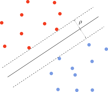
Let’s say we are in two dimensions, and we have a dataset with two labels. We want to find the line that achieves maximal separation between the two classes. That is, of all the separating lines, we want to find the one that maximizes the margin $\rho$, as depicted below.

A line has equation \(\omega^T\cdot x+b=0\) where $x=(x_1,x_2)$ are the 2d coordinates and $\omega$ is the normal vector. The distance between a point with coordinates $x$ and the line is given by $\omega^T(x-x_0)/{\lVert\omega\rVert}$, where $x_0$ is a point on the plane. Since $\omega^T\cdot x_0=-b$, the signed distance is \(d=\frac{\omega^T\cdot x+b}{\lVert\omega\rVert}\)
The margin is defined as a the minimum distance $C$ from the separating line, that is, $C=\text{Min }{y_i d_i}$. The optimal separating line maximizes this margin, that is, \(y_i\frac{\omega^T\cdot x_i+b}{\lVert\omega\rVert}\geq \text{Max }C=\rho,\;\forall (x_i,y_i)\) We have multiplied by the target $y_i\in{-1,1}$ to guarantee that each term is always positive on both sides of the separating line. Since the line equation is invariant under rescaling $(\omega,b)\rightarrow (\lambda \omega,\lambda b)$ we can choose $\lVert\omega\rVert=1/\rho$. This means that maximizing $\rho$ as above is equivalent to \(\text{Min }\lVert\omega\rVert,\;\;y_i(\omega^T\cdot x_i+b)\geq 1,\;\forall (x_i,y_i)\)
We can translate this minization problem to finding the minima of the loss function \(L=\frac{1}{2}\sum_{k=1}^d \omega_k^2 -\sum_{i=1}^N\alpha_i[ y_i(\omega^T\cdot x_i+b)-1],\;\alpha_i\geq 0\) where $\alpha_i$ are Lagrange multipliers, $d$ is the number of dimensions and $N$ is the number of datapoints. The local minima solves the equations
\[\begin{equation*}\begin{split}&\frac{\partial L}{\partial \omega_k}=\omega_k -\sum_{i=1}^N\alpha_i y_ix^k_i=0\\ &\frac{\partial L}{\partial b}=\sum_i\alpha_iy_i=0\\ &\frac{\partial L}{\partial \alpha_i}= y_i(\omega^T\cdot x_i+b)-1=0 \end{split}\end{equation*}\]Provided $\alpha_i>0$ for which the loss function is differentiable in $\alpha$. If $\alpha_i=0$ then the we only have the first two equations. This means that $\alpha_i>0$ corresponds to points that sit exactly on the margin, and the remaining equations depend only on these points. These are known as support vectors.
If we replace $\omega$ with its equation in the loss function $L$, we obtain the dual problem:
\[\hat{L}=\sum_{i=1}^N\alpha_i-\frac{1}{2}\sum_{i=1}^N\sum_{j=1}^N\alpha_i \alpha_j y_iy_j x_i^T\cdot x_j,\;\alpha_i\geq 0\]where we have used that $\sum_i\alpha_iy_i=0$. The problem with $-\hat{L}$ is actually a convex minimization problem and can be solved using traditional methods. The solution of the dual problem must suplemented with the additional conditions:
\[\begin{equation*}\begin{split}&y_i(\omega^T\cdot x_i+b)=1,\;\alpha_i>0\\ &y_i(\omega^T\cdot x_i+b)>1,\;\alpha_i=0\\ &\sum_i\alpha_i y_i=0\end{split}\end{equation*}\]Support vectors live on the margin and thus $y_i(\omega^T\cdot x_i+b)=1$. Given a support vector $x_s,y_s$, we can use this equation to determine $b$ \(b=y_s-\sum_{i=1}^m\alpha_p y_px_p^T\cdot x_s\) where $p=1\ldots m$ runs over the support vectors. $\hat{L}$ is maximized by the solution and as such \(\frac{\partial\hat{L}}{\partial \alpha_s}=1-y_s\sum_{p=1}^m\alpha_py_px_p^T\cdot x_s=0\) Multiplying this equation by $\alpha_s$ and summing over $s$ we obtain
\[\sum_{s=1}^m\alpha_s-\sum_{s=1}^m\sum_{p=1}^m\alpha_s\alpha_py_sy_px_p^T\cdot x_s=0\iff \lVert\omega\rVert^2=\sum_{s=1}^m\alpha_s=\lVert\alpha\rVert_1\]So the margin is inversely proportional to the linear norm of $\alpha$.
- Non-separable case:

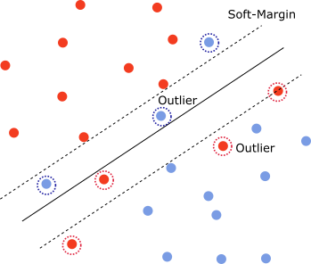
In the non-separable case, one cannot find a hyperplane that separates the classes. That is, for any hyperplane, there exists $x_i,y_i$ such that
\[y_i(\omega^T\cdot x_i +b)\ngtr 1\]See picture above.
However, one can formulate a relaxed version of the constraints using slack variables $\xi_i\geq 0$
\[y_i(\omega^T\cdot x_i +b)\geq 1-\xi_i\]If we remove the points for which $0 < y_i(\omega^T\cdot x_i +b)<1$ then the data is linearly separable. With the remaining data, we can define a margin called a soft-margin instead of a hard-margin as in the separable case. The points for which $\xi_i$ is non-zero are the outliers.
As before, we want to minimize $\lVert\omega\rVert$, but at the same time we want to use the smallest possible number of $\xi$ with the smallest values possible. This can be written as
\[\frac{1}{2}\lVert\omega\rVert^2+\lambda \sum_i \xi_i^p-\sum_i\alpha_i[y_i(\omega^T\cdot x_i +b)- 1+\xi_i],\;\alpha_i\geq 0,\xi_i\geq 0\]The term $\lambda \sum_i \xi_i^p$ with $\lambda>0$ works as a regulator, which prevents $\xi_i$ from taking large values as well as having a large number of non-zero $\xi_i$. The exponent $p$ defines different types of regularization. For $p=1$ the loss function becomes the Hinge loss function
\[\frac{1}{2}\lVert\omega\rVert^2+\lambda\sum_i \text{max}(0,1-y_i(\omega^T\cdot x_i +b))\]The next steps are very similar to the separable case. One can build a dual problem and determine the support vectors and outliers.
2. Generalization properties
Given the separating hyperplane we can build the predictor
\[h(x)=\text{sign}(\omega\cdot x+b)\]We want to bound the generalization error
\[R(h_S)=\sum_{x,y} 1_{h(x)\neq y}D(x)\]To do this we can explore the leave-one-out error $R_{LOO}$. The $R_{LOO}(x)$ is the error on a point $x$ provided we train the algorithm on the remaining $S\setminus{x}$ dataset, that is, with the point $x$ excluded. The empirical $\hat{R}_{LLO}$ is obtained by averaging over all points of the dataset $S$, that is,
\[\hat{R}_{LLO}=\frac{1}{m}\sum_{x} R_{LLO}(x)\]One can show that the average of $\hat{R}_{LLO}$ is an unbiased estimate of the generalization error. That is,
\[\mathbb{E}_{S\sim D^m} \hat{R}_{LLO}=\mathbb{E}_{S'\sim D^{m-1}}(R(h_{S'}))\]In more detail,
\[\begin{aligned}\mathbb{E}_{S\sim D^m} \hat{R}_{LLO}&=\mathbb{E}_{S\sim D^m}\frac{1}{m}\sum_{x} R_{LLO}(x)\\ &=\mathbb{E}_{S\sim D^m}1_{h_{S'}(x)\neq y}\\ &=\mathbb{E}_{S'\sim D^{m-1},x\sim D}1_{h_{S'}(x)\neq y}\\ &=\mathbb{E}_{S'\sim D^{m-1}}R(h_{S'}) \end{aligned}\]Let’s estimate $R_{LLO}(x)$ for the SVM in the separable case. If $x$ is above the margin, then the error is zero because if we remove this point, the predictor will not change as it depends only on the support vectors. However, if $x$ is exactly on the margin, then the new predictor’s support vectors will change. This point $x$ may or may not be correctly classified, and so the maximum number of points that this procedure can misclassify is the same as the number of support vectors. This means that, \(\hat{R}_{LLO}\leq \frac{NV(S)}{m}\) where $NV$ is the number of support vectors for the dataset $S$. We may therefore conclude that the average generalization error is bounded by the average number of support vectors, that is, \(\mathbb{E}_{S'\sim D^{m-1}}R(h_{S'})\leq \frac{\mathbb{E}_{S\sim D^m}NV(S)}{m}\)
Assuming that $NV$ remains small for different datasets, the above result implies that the average error remains small.
3. Non-linear decision boundary
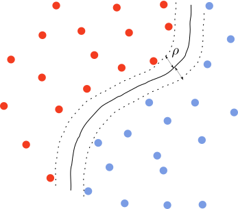
The dataset may be separable, but the decision boundary is not a hyperplane. In this case, there should exist a map $\phi: x\rightarrow x’$ that makes the problem linearly separable. All the previous steps follow except that we use $x’$ instead of $x$. The problem is in determining the map $\phi$, which is usually a difficult problem.

Kernel methods are used to address solutions of this type. Suppose we find such a map. Then we have a new set of features $\phi(x_1),\phi(x_2),\ldots \phi(x_n)$. The dual problem becomes
\[L_D=\sum_{i=1}^N\alpha_i-\frac{1}{2}\sum_{i=1}^N\sum_{j=1}^N\alpha_i \alpha_j y_iy_j \phi(x_i)^T\cdot \phi(x_j),\;\alpha_i\geq 0\]and the predictor
\[\begin{equation*}\begin{split}G(x)&=\text{sign} \big(\omega^T\phi(x)+b\big)\\ &=\text{sign} \big(\sum_{i=1}^N\alpha_i y_i\phi(x)^T\cdot\phi(x_i)+b\big) \end{split}\end{equation*}\]The constant $b$ can be determined from the location of a support vector. So we see that the solution only depends on the scalar $K(x,x’)=\phi(x)^T\cdot \phi(x’)$. The function $K(x,x’)$ is a Kernel function and obeys the following conditions
- It is symmetric: $K(x,x’)=K(x’,x)$
- It is positive semi-definite: $\sum_{i,j}K(x_i,x_j)\lambda_i\lambda_j\geq 0,\; \forall \lambda_i$
Instead of looking for the map $\phi$, we can search for the Kernel, a scalar function. For example, let’s consider the gaussian Kernel: \(K(x,y)=e^{-\frac{\lVert x-y\rVert^2}{2\sigma^2}}\) Since this is a positive and symmetric function, it is easy to see that the above conditions are satisfied. But can we find the map $\phi$ such that $K(x,x’)=\phi(x)^T\phi(x’)$? Note that
\[e^{-\frac{\lVert x-y\rVert^2}{2\sigma^2}}=e^{-\frac{x^2+y^2}{2\sigma^2}}\sum_{n=1}^{\infty}\frac{(xy)^n}{(2\sigma^2)^n n!}\]For each polynomial term in the expansion
\[\begin{equation*}\begin{split}(x y)^n=(\sum_{i=1}^d x_iy_i)^n&=\sum_{\sum_i k_i=n}\frac{n!}{k_1!k_2!\ldots k_d!}(x_1y_1)^{k_1}(x_2y_2)^{k_2}\ldots (x_dy_d)^{k_d}\\ &=\sum_{\sum_i k_i=n}\frac{n!}{k_1!k_2!\ldots k_d!} x_1^{k_1}x_2^{k_2}\ldots x_d^{k_d} y_1^{k_1}y_2^{k_2}\ldots y_d^{k_d}\\ &=h_n(x)^T\cdot h_n(y) \end{split}\end{equation*}\]where
\[h_n(x)=(x_1^n,\sqrt{n} x_1^{n-1}x_2,\sqrt{n} x_1^{n-1}x_3,\ldots,\sqrt{\frac{n!}{k_1!k_2!\ldots k_d!}} x_1^{k_1}x_2^{k_2}\ldots x_d^{k_d},\ldots x_d^n)\]This means that for the gaussian Kernel the map $\phi$ is infinite dimensional. This shows how powerful Kernel methods can be.
4. Python implementation
- The CVXOPT library can be used to solve quadratic optimization problems with constraints.
import cvxopt

class LinearSVM:
    def __init__(self,num_iter=10**5):

        self.coef_=None
        self.intercept_={}
        self.weight_={}
        self.support_vectors_={}
        self.classes=None
        self.num_iter=num_iter

    def fit(self,x,y):
        y_aux=y.copy().reshape(-1,1)
        y_aux=y_aux.astype('float64')
        self.classes=set(y)

        cvxopt.solvers.options['show_progress'] = False

        pairs=[[(i,j)  for i in self.classes for j in self.classes if j>i]]

        for i,j in pairs:
            idx=(y_aux==i) | (y_aux==j)
            idx=idx.reshape(-1,)
            x_temp=x[idx].copy()
            y_temp=y_aux[idx].copy()
            y_temp[y_temp==j]=-1.0
            y_temp[y_temp==i]=1.0

            z=y_temp*x_temp
            Q=0.5*np.tensordot(z,z,axes=[(1),(1)])
            Q=cvxopt.matrix(Q.tolist())
            p=-1*np.ones(x_temp.shape[0])
            p=cvxopt.matrix(p.tolist())
            G=-1*np.identity(x_temp.shape[0])
            G=cvxopt.matrix(G.tolist())
            h=np.zeros(x_temp.shape[0])
            h=cvxopt.matrix(h.tolist())
            A=cvxopt.matrix(y_temp.tolist())
            b=cvxopt.matrix(0.0)

            sol=cvxopt.solvers.qp(Q, p, G, h, A, b)
            sol=np.array(sol['x'])

            #support vectors
            sup_vec_loc=np.round(sol,2).reshape(-1,)
            sol[sup_vec_loc==0]=0
            sup_vec_loc=sup_vec_loc!=0
            sup_vec=x_temp[sup_vec_loc]
            self.support_vectors_[pair]=sup_vec

            #margin
            w=((sol*y_temp)*x_temp).sum(0)
            y_s=y_temp[sup_vec_loc]
            v=np.dot(sup_vec,w.reshape(-1,1))
            coef=(y_s*v).mean()-y_s.mean()*v.mean()
            coef=coef/(v.var())
            intercept=y_s.mean()-coef*v.mean()

            self.intercept_[pair]=intercept
            self.weight_[pair]=coef*w
- SMO algorithm
In the SMO algorithm, or sequential minimal optimization, we solve the dual minimization problem iteratively. First we randomly initialize all $\alpha_i$. Then we choose a random pair of $\alpha$’s, say $\alpha_0,\alpha_1$ and solve for the minimum of $L(\alpha_0,\alpha_1)$ with the other $\alpha$ fixed. This is easy to do because the function $L(\alpha_0,\alpha_1)$ is actually one dimensional after using the constraint $\sum_i \alpha_i y_i=0$. Then we proceed with a different pair of $\alpha$’s and repeat until the solution converges.
"""Ensure that the target y has values -1,1
    Step 1): generate all (i,j) to get access to alpha pairs
    Step 2):
"""
alpha=np.random.normal(0,10,(y.shape[0],1))
alpha=np.abs(alpha)

l=[i for i in range(x.shape[0])]
samples=[(i,j) for i in l for j in l if i<j]
random.shuffle(samples)

num_iter=0
threshold=len(samples)
alpha_prev=alpha.copy()
T=(alpha*y).sum()
Z=(alpha*y*x).sum(0)

not_converged=True
while not_converged and num_iter<5*threshold:

    for i,j in samples:

        alpha0=alpha[i][0]
        alpha1=alpha[j][0]
        y0=y[i][0]
        y1=y[j][0]

        #If constraint is possible to be solved continue
        k=-T+alpha0*y0+alpha1*y1
        if y1*k<0 and y0*y1>0:
            continue

        # Solve 2-dimensional optimization problem with constraint
        A=Z-alpha0*y0*x[i]-alpha1*y1*x[j]
        B=x[i]-x[j]
        a=1-y0*y1-y0*k*np.dot(B,x[j])-y0*np.dot(B,A)
        a=a/(np.dot(B,B))

        alpha0=max(0,a)
        alpha1=y1*k-alpha0*y0*y1
        if alpha1<0:
            alpha1=0
            alpha0=k*y0

        #update alpha
        alpha[i][0]=alpha0
        alpha[j][0]=alpha1

        T=-k+alpha0*y0+alpha1*y1
        Z=A+alpha0*y0*x[i]+alpha1*y1*x[j]

        # verify if alpha converges
        error=alpha-alpha_prev
        error=np.abs(error).max()
        if error<10**(-8) and num_iter>3*threshold:
            not_converged=False
            print('converged')
            break
        alpha_prev=alpha.copy()
        num_iter+=1
References
[1] Understanding Machine Learning: from Theory to Algorithms, Shai Ben-David and Shai Shalev-Shwartz
[2] The elements of statistical learning, T. Hastie, R. Tibshirani, J. Friedman
[3] Foundations of machine learning, M. Mohri, A. Rostamizadeh, A. Talwalkar