Neural Network
- 1. Neural Network
- 2. Backpropagation
- 3. VC-dimension
- 4. Decision Boundary
- 5. Python implementation
- References
1. Neural Network
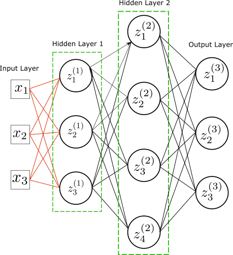
A neural network is a graph composed of nodes and edges. The edges implement linear operations while the nodes aggregate each edge’s contribution before composing by an activation function $g$. This process is replicated to the next layer. Note that the nodes do not interact with each other within each layer; that is, there is no edge between nodes. Mathematically we have the following series of operations.
\[\begin{equation}\begin{split}&z^{(l)}_i=g(\omega^{(l)}_{ij}z^{(l-1)}_j+b^{(l)}_j)\\ &z^{(l-1)}_j=g(\omega^{(l-1)}_{jk}z^{(l-2)}_k+b^{(l-1)}_j)\\ &\ldots\\ &z^{(1)}_p = g(\omega^{(1)}_{pr}x_r+b^{(0)}_l) \end{split}\end{equation}\]The activation function $g$ is a non-linear function with support on the real line. A common choice is the sigmoid function but the sign function also works. This sequence of compositions is known as forward pass.
A neural network is a type of universal approximator. Cybenko (1989) has shown that any continuous function $f$ in $I_n$, the n-dimensional unit cube, can be approximated with arbitrary accuracy by a sum of the form \(C=\sum_{i=1}^N \alpha_i\sigma(\beta_i^T\cdot x+b_i)\) That is, \(|C(x)-f(x)|<\epsilon,\;\forall x\in I_n\) for any $\epsilon>0$.
The network architecture has two major parameters that we need to tune: the number of neurons per layer and the depth or number of layers. Increasing the number of neurons in a layer adds complexity to the neural network because we add more parameters to fit. And the depth does it too. However, adding depth to the neural network increases the number of parameters more rapidly than adding neurons in the same layer. Suppose we have one hidden layer with $n$ neurons. The number of edges flowing to this layer is $n(d+1)$ where $d$ is the input dimension. Instead, if we consider two hidden layers with $n/2$ neurons each, we have in total $n(n/2+1)/2+n(d+1)/2$ edges flowing to the hidden layers. This number scales quadratically with $n$, while for a single hidden layer, it scales linearly.
But adding depth has an additional effect. We can see the output of a layer as a different feature representation of the data. Adding layers also allows the neural network to learn other representations of the data, which may help performance. The neural network can be trained beforehand on large datasets and learn very complex features. We can take the last hidden layer as a new input feature and train only the last layer weights. Training the last layer allows the neural network to learn datasets that may differ, in population, from the training set.
Instead, if we were to train a neural network with only one hidden layer, we would need to add an increasing number of neurons to capture more complex functions. However, the effect of having a large number of neurons may be prejudicial as we are increasing the dimension of the hidden feature space, leading to dimensionality issues. In contrast, adding depth increases complexity while keeping the dimensionality of the hidden space under control.
Although depth helps to learn, it brings other shortcomings in terms of training. With more depth, the loss function derivatives can be challenging to calculate. While the last layers’ parameters are easier to learn, the first layers’ parameters can be hard to learn. Having many products will eventually make the derivative approach zero or become quite large, which hinders training.
2. Backpropagation
Lets consider a binary classification problem with classes $y={0,1}$. In this case we want to model the probability $p(x)\equiv p(y=1|x)$. The loss function is the log-loss function given by
\[L=-\sum_iy_i\ln p(x_i)+(1-y_i)\ln(1-p(x_i))\]and we model $p(x)$ with a neural network with one hidden layer, that is,
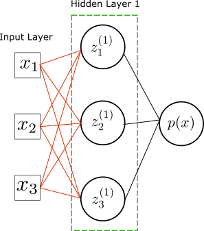
So we have
\[\begin{aligned}& p(x)=\sigma(\omega^{(2)}_{i}z^{(1)}_i+b^{(2)})\\ &z^{(1)}_j = \sigma( \omega^{(1)}_{jk}x_k+b^{(1)}_j) \end{aligned}\]where implicit contractions are in place.
The loss function depends on the weights \(\omega^{(2)}_i\) and \(\omega^{(1)}_{ij}\) in a very complicated way. To calculate the minimum of the loss function we use the gradient descent algorithm. So we calculate the derivatives of the loss function with respect to the weights,
\[\begin{equation*}\begin{split}&\frac{\partial L}{\partial \omega^{(2)}_i}=\sum_x \frac{\partial L}{\partial p(x)}\dot{\sigma}(\omega^{(2)}_{k}z^{(1)}_k+b^{(2)})z^{(1)}_i\\ &\frac{\partial L}{\partial b^{(2)}}=\sum_x \frac{\partial L}{\partial p(x)}\dot{\sigma}(\omega^{(2)}_{k}z^{(1)}_k+b^{(2)})\\ &\frac{\partial L}{\partial \omega^{(1)}_{ij}}=\sum_x \frac{\partial L}{\partial p(x)}\dot{\sigma}(\omega^{(2)}_{k}z^{(1)}_k+b^{(2)})\omega^{(2)}_i \dot{\sigma}(\omega^{(1)}_{ik} x_k+b^{(1)}_i)x_j\\ &\frac{\partial L}{\partial b^{(1)}_{i}}=\sum_x \frac{\partial L}{\partial p(x)}\dot{\sigma}(\omega^{(2)}_{k}z^{(1)}_k+b^{(2)})\omega^{(2)}_i \dot{\sigma}(\omega^{(1)}_{ik} x_k+b^{(1)}_i) \end{split}\end{equation*}\]We see that as we go down in the layer level, we need to propagate back the composition of the forward pass in order to calculate the derivatives. That is, first we calculate the derivatives of the weights in the higher levels, and progress downwards towards lower levels. This process can be done in an iterative way, and is known as backpropagation algorithm. More generally we have
\[\begin{equation*}\begin{split}&\frac{\partial p_k(x)}{\partial \omega^{(n)}_{ij}}=\dot{g}^{(l)}_k\omega^{(l)}_{kk_1} \dot{g}^{(l-1)}_{k_1}\omega^{(l-1)}_{k_1k_2}\ldots \dot{g}^{(n)}_i z^{(n-1)}_j\\ &\frac{\partial p_k(x)}{\partial b^{(n)}_{i}}=\dot{g}^{(l)}_k\omega^{(l)}_{kk_1} \dot{g}^{(l-1)}_{k_1}\omega^{(l-1)}_{k_1k_2}\ldots \dot{g}^{(n)}_i \end{split}\end{equation*}\]where again sums over indices are implicit.
3. VC-dimension
We can estimate the VC-dimension of a neural network with activation the sign function. Recall the growth function definition: $\text{max}_{C\in \chi: |C|=m}|\mathcal{H}_C|$ where $\mathcal{H}_C$ is the restriction of the neural network hypotheses from the set $C$ to ${0,1}$. Between adjacent layers $L^{t-1}$ and $L^{t}$ one can define a mapping between $\mathcal{H}^t:\,\mathbb{R}^{|L^{t-1}|}\rightarrow \mathbb{R}^{|L^{t}|}$, where $|L^{t-1}|$ and $|L^t|$ are the number of neurons in the layers, respectively. Then the hypothesis class can be written as the composition of each of these maps, that is, $\mathcal{H}=\mathcal{H}^T\circ \ldots \circ \mathcal{H}^1$. The growth function can thus be bounded by \(\Pi_{\mathcal{H}}(m)\leq \prod_{t=1}^T\Pi_{\mathcal{H^t}}(m)\)
In turn, for each layer the class $\mathcal{H}^t$ can be written as the product of each neuron class, that is, $\mathcal{H}^t=\mathcal{H}^{t,1}\times \ldots \times \mathcal{H}^{t,i}$ where $i$ is the number of neurons in that layer. Similarly, we can bound the growth function of each layer class \(\Pi_{\mathcal{H}^t}(m)\leq \prod_{i=1}^{|L^t|}\Pi_{\mathcal{H^{t,i}}}(m)\)
Each neuron is a homogeneous halfspace class, and we have seen that the VC-dimension of this class is the dimension of their input plus one (VC-dimension of a separating hyperplane). If we count the bias constant as a single edge, then this dimension is just the number of edges flowing into the node $i$, which we denote as $d_{t,i}$. Using Sauer’s Lemma, we have \(\Pi_{\mathcal{H}^{t,i}}\leq \Big(\frac{em}{d_{t,i}}\Big)^{d_{t,i}}<(em)^{d_{t,i}}\)
Putting all these factors together we obtain the bound \(\Pi_{\mathcal{H}}(m)\leq \prod_{t,i} (em)^{d_{t,i}}=(em)^{|E|}\) where $|E|$ is the total number of edges, which is also the total number of parameters in the network. For \(m^*=\text{VC-dim}\) we have \(\Pi_{\mathcal{H}}=2^{m^*}\) , therefore \(2^{m^*}\leq (em^*)^{|E|}\) It follows that $m^*$ must be of the order $\mathcal{O}(|E|\log_2|E|)$.
If the activation function is the sigmoid, the proof is out of scope. One can though give a rough estimate. The VC-dimension should be of the order of the number of tunable parameters. This is the number of edges \(|E|\), counting the bias parameters.
4. Decision Boundary
Below we plot the decision boundary for a neural network with one hidden layer after several iterations, that is, the number of gradient descent steps:
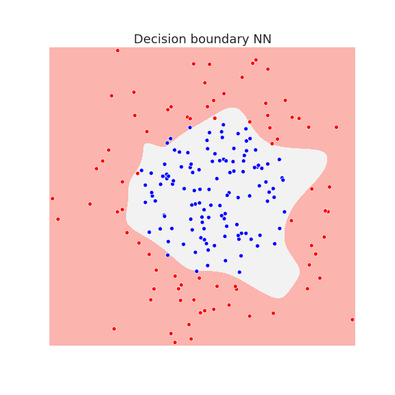
The neural network has enough capacity to draw complicated decision boundaries. Below we show the decision boundary at different stages of learning.
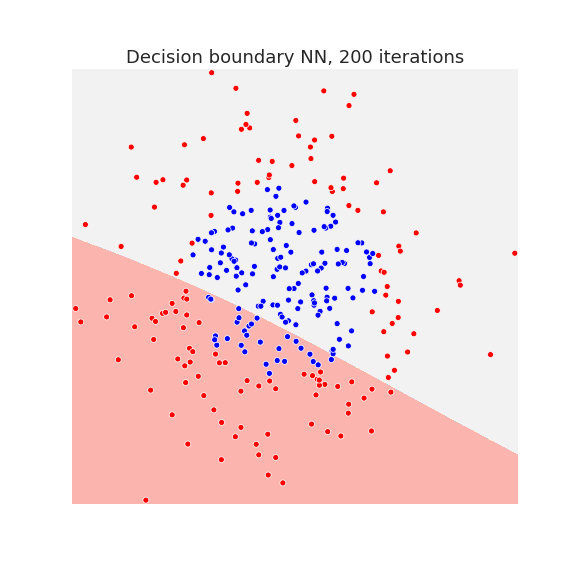
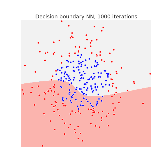
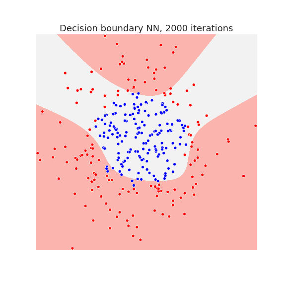
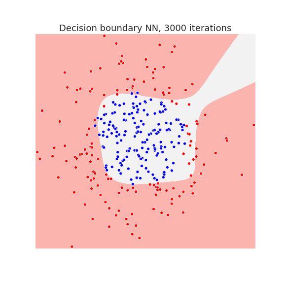
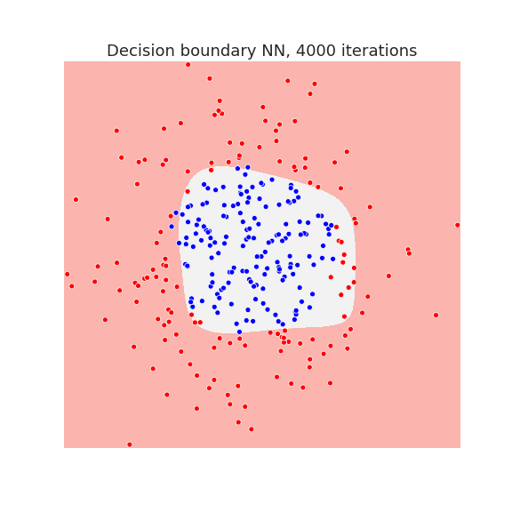
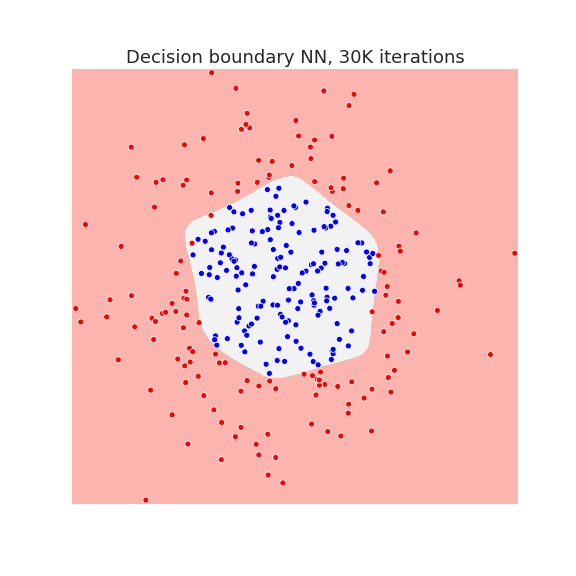
Waiting long enough, allows the neural network to overfit the data as we see in the last picture.
5. Python implementation
Define classes for linear layer and sigmoid activation function:
class LinearLayer:
    def __init__(self,dim_in,dim_out):
        self.n_in=dim_in
        self.n_out=dim_out
        self.weights=np.random.normal(0,0.01,(dim_in,dim_out))
        self.bias=np.random.normal(0,0.01,dim_out)

    def __call__(self,x):
        out=np.matmul(x,self.weights)
        out+=self.bias

        return out

    def backward(self,x):
        dL=x

        return dL

class Sigmoid:
    "sigmoid function"

    def __call__(self,x):
        out=1/(1+np.exp(-x))

        return out

    def backward(self,x):
        out=np.exp(-x)/(1+np.exp(-x))**2
        return out
Class NN: implements neural network
Class logloss: returns loss function object which contains backward derivates for gradient descent
Class optimizer: implements gradiend descent step with specified learning rate
class NN:
    """ Neural Network with one hidden layer"""

    def __init__(self,dim_in,hidden_dim,dim_out):
        self.layer1=LinearLayer(dim_in,hidden_dim)
        self.layer2=LinearLayer(hidden_dim,dim_out)
        self.sig=Sigmoid()
        self.delta=None

    def __call__(self,x):
        self.out_l1=self.layer1(x)
        self.out_s1=self.sig(self.out_l1)
        self.out_l2=self.layer2(self.out_s1)
        self.out_s2=self.sig(self.out_l2)

        return self.out_s2

    def predict(self,x):
        p=self(x)

        pred=(p>=0.5).astype('int')

        return pred

class logloss:

    def __init__(self,model):
        self.model=model

    def __call__(self,x,y):
        p=self.model(x)
        L=y*np.log(p)+(1-y)*np.log(1-p)

        return -L.sum()/x.shape[0]

    def backward(self,x,y):
        p=self.model(x)
        dL=-y/p+(1-y)/(1-p)
        dL=dL/x.shape[0]
        dL=dL*model.sig.backward(model.out_l2)
        dw2,db2=np.dot(model.out_s1.T,dL),dL.sum()

        dw1=model.layer2.weights.T*model.sig.backward(model.out_l1)
        db1=(dL*dw1).sum(0)
        dw1=np.dot((dL*x).T,dw1)

        model.delta=db1,dw1,db2,dw2

class optimizer:

    def __init__(self,model,lr=0.01):
        self.model=model
        self.lr=lr

    def step(self):

        db1,dw1,db2,dw2=model.delta
        self.model.layer1.bias-=db1*self.lr
        self.model.layer1.weights-=dw1*self.lr
        self.model.layer2.bias-=db2*self.lr
        self.model.layer2.weights-=dw2*self.lr
Training for loop:
def train(optimizer,loss,xtrain,ytrain,num_iter=100):

    for i in range(num_iter):

        L=loss(xtrain,ytrain)
        loss.backward(xtrain,ytrain)
        optimizer.step()

        if i%10==0:
            print('Iteration ',i,', loss: ',L)
References
[1] Understanding Machine Learning: from Theory to Algorithms, Shai Ben-David and Shai Shalev-Shwartz
[2] The elements of statistical learning, T. Hastie, R. Tibshirani, J. Friedman
[3] Approximation by superpositions of a sigmoidal function, Cybenko, G. (1989)