Boltzmann Machine
1. Boltzmann Machine
A Boltzmann machine models an unsupervised probability distribution using a graphical representation composed of visible and hidden units. The visible data’s probability is obtained by summing over the hidden variables, with a weight function, which is the exponential of the energy term \(E(v,h)\), like the Boltzmann distribution in statistical mechanics. For the diagram below
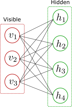
the probability has the form
\[P(v)=\sum_{\{h\}}P(v,h)=\sum_{\{h\}}\frac{\exp{E(v,h)}}{Z}=\sum_{\{h\}}\frac{\exp{(-\sum_iv_ia_i-\sum_ih_ib_i-\sum_{i,j}v_iW_{ij}h_j)}}{Z}\]where the sum is over all hidden configurations \(h=\{0,1\}^d\), with $d$ the dimension of the hidden layer. The parameters $a,b$ are the biases and \(W_{ij}\) is a matrix representing the interactions between the visible and hidden layers. The visible unit is composed of binary features \(v_i=\{0,1\}\). The normalization \(Z\) is the partition function
\[Z(a,b,W)=\sum_{v,h}P(v,h)\]The Boltzmann machine can have more complicated graph interaction including edges between both visible and hidden units. For example
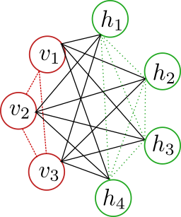
A restricted Boltzmann machine is a Boltzmann machine for which there are no interactions between the nodes in the same layer. In terms of parameters, each node $i$ contains a bias \(b_i\), and a parameter \(W_{ij}\) for each edge between the nodes \(i\) and \(j\).
2. Training
During training, we want to minimize the Kullback-Leibler divergence between the actual distribution of visible data \(D(v)\) and the output of the Boltzmann machine \(P(v)\). That is, we seek the optimum of
\[\begin{equation*}\begin{split}KL(D||P)=\sum_v D(v)\ln\Big(\frac{D(v)}{P(v)}\Big)\end{split}\end{equation*}\]Lets focus for the moment on a restricted machine with one hidden layer. The derivatives of the loss function \(L\equiv KL(D||P)\) with respect to the weights is
\[\begin{equation}\begin{split}\frac{\partial L}{\partial W_{ij}}&=\sum_v D(v)\frac{\sum_h v_ih_j \exp{E(v,h)}}{\sum_h \exp{E(v,h)}}-\sum_v D(v)\frac{\sum_{v',h'}v'_ih'_j \exp{E(v',h')}}{Z}\\ &=\sum_{v,h} v_ih_j P(h|v)D(v) -\sum_{v,h}v_ih_j P(v,h)\\ &=\langle v_ih_j\rangle_{data}-\langle v_ih_j\rangle_{model}\end{split}\end{equation}\]and similarly for the biases
\[\begin{equation*}\begin{split}&\frac{\partial L}{\partial a_{i}}=\langle v_i\rangle_{data}-\langle v_i\rangle_{model}\\&\frac{\partial L}{\partial b_{i}}=\langle h_i\rangle_{data}-\langle h_i\rangle_{model}\end{split}\end{equation*}\]Since the gradient is the sum of two averages, one can use stochastic optimization. To calculate \(\langle hv\rangle_{data}\) we can generate unbiased samples \(h_iv_j\) and then take the average as an estimate. To do that, we can use Gibbs sampling. First we pick a training sample \(v\) and then generate a sample \(h\) using the conditional probability \(P(h_1,h_2,\ldots|v)\) . We can write
\[\begin{equation*}\begin{split}P(h_1,h_2,\ldots|v)&=\frac{P(h_1,h_2,\ldots,v)}{\sum_h P(h,v)}=\\ &=\frac{\exp{(-\sum_j h_jb_j -\sum_{ij}v_iW_{ij}h_j)}}{\prod_{j}(1+\exp{(-b_j-\sum_{i}v_i W_{ij})})}\\ &=\prod_j\frac{\exp{(-h_jb_j -h_j\sum_{i}v_iW_{ij})}}{(1+\exp{(-b_j-\sum_{i}v_i W_{ij})})}\\ &=\prod_{j=1}^{N_h} P(h_j|v)\end{split}\end{equation*}\]where \(N_h\) is the number of hidden units and we have defined
\[P(h_j=1|v)=\frac{1}{1+\exp{(b_i+\sum_i v_iW_{ij})}}\]Similarly the probability \(P(v_1,v_2,\ldots|h)\) can be written as
\[P(v_1,v_2,\ldots|h)=\prod_{i=1}^{N_v} P(v_i|h)\]where \(N_v\) is the number of visible units and
\[P(v_i=1|h)=\frac{1}{1+\exp{(a_i+\sum_j W_{ij}h_j)}}\]The probabilty for visible states can also be written in a compact way. Defining
\[\begin{equation*}\begin{split}\Phi(v)&\equiv\sum_{h}\exp{(-\sum_i v_i a_i-\sum_j h_j b_j-\sum_{ij}v_iW_{ij}h_j)}=\\ &=\exp{(-\sum_i v_i a_i)}\prod_{j}(1+\exp{(-b_j-\sum_{i}v_i W_{ij})})\end{split}\end{equation*}\]this probability becomes
\[P(v)=\frac{\Phi(v)}{\sum_v \Phi(v)}\]However, to generate a sample for the average \(\langle hv\rangle_{model}\) is quite harder because we do not have direct access to \(P(v)\). Instead choose a training vector \(v\) and generate a state \(h\) using \(P(h|v)\). Further, given this state \(h\) reconstruct the state \(v\) using \(P(v|h)\). The change in the weight is then given by
\[\Delta W_{ij}=-\eta( \langle v_ih_j\rangle_{data}-\langle v_ih_j\rangle_{recons})\]where \(\eta\) is the learning rate.
If the Boltzmann machine contains couplings between nodes in the same layer, the analysis is very similar. We calculate the derivatives of the loss with respect to \(L_{ij}\) and \(J_{ij}\), respectively the couplings between visible-visible and hidden-hidden units,
\[\begin{equation*}\begin{split}&\frac{\partial L}{\partial L_{ij}}=\langle v_iv_j\rangle_{data}-\langle v_iv_j\rangle_{model}\\&\frac{\partial L}{\partial J_{ij}}=\langle h_ih_j\rangle_{data}-\langle h_ih_j\rangle_{model}\end{split}\end{equation*}\]Again the idea is to replace the model average with a point estimate by generating unbiased samples \(v_iv_j\) and \(h_ih_j\) and calculate their sample averages.
To monitor training, we usually plot values of the log-likelihood function. However, in a Boltzmann machine determining the probability \(P(v)\) is prohibitively expensive since calculating the partition function \(Z\) requires adding up an exponential number of terms. The complexity is of order \(\mathcal{O}(2^{N_v})\), where \(N_v\) is the number of visible units. Instead, we calculate the pseudo-loglikelihood. This quantity is defined as
\[\text{Pseudo-LL}(v)=\sum_{i}\ln P(v_i|\{v_{j\neq i}\})\]that is, the sum over the log-probabilities conditioned on the remaining visible units. Remember that the log-likelihood can be written as
\[\ln P(v)=\ln P(v_1)+\ln P(v_2|v_1) +\ln P(v_3|v_1,v_2)+\ldots+\ln P(v_n|\{v_{1:n-1}\})\]after using the Bayes theorem. It can be shown that the pseudo-loglikelihood descreases during training.
3. Python implementation
We use the MNIST dataset for a python experiment on Boltzmann machines. The dataset consists of 70000 images of handwritten digits, from 0 to 9. Each image contains \(28\times 28=784\) pixels ranging from 0 to 255. If we work with normalized pixels, then we can interpret that value as the probability of being white or black. We can then generate a set of binary states by drawing zeros or ones according to each pixel probability. Once the model is trained, we can generate samples of visible states using Gibbs sampling. First, we take a random set of visible states \(v^0\), and then we use \(P(h|v^0)\) to generate a sample of hidden states \(h^0\). Given this hidden state, we can sample a new set of visible states \(v^1\) using \(P(v|h^0)\).
- RBM class
class RBM:
    def __init__(self,vis_dim,hidden_dim):
        self.vis_dim=vis_dim
        self.hidden_dim=hidden_dim
        self.weight=np.random.normal(0,0.001,(vis_dim,hidden_dim))
        self.bias_vis=np.random.normal(0,0.001,vis_dim)
        self.bias_hid=np.random.normal(0,0.001,hidden_dim)

    def prob_h_v(self,vis_vec):

        probs=1+np.exp(self.bias_hid+np.matmul(vis_vec,self.weight))

        return 1/probs

    def prob_v_h(self,hid_vec):

        probs=1+np.exp(self.bias_vis+np.matmul(hid_vec,self.weight.T))

        return 1/probs

    def Pv(self,vis_vec):

        self.Z()
        p=self.__phi(vis_vec)/self.Z_

        return p

    def __phi(self,vis_vec):

        p=np.exp(-np.matmul(vis_vec,self.bias_vis))
        t=1+np.exp(-self.bias_hid-np.matmul(vis_vec,self.weight))
        p=p*np.prod(t,axis=1)

        return p

    def pseudoLL(self,X):

        phis=self.__phi(X)
        pseudo=np.zeros(X.shape[0])
        temp=X.copy()
        for i in range(X.shape[1]):
            #flip
            temp[:,i]=np.abs(temp[:,i]-1)
            Z=phis+self.__phi(temp)
            pseudo+=np.log(phis/Z)
            #flip again
            temp[:,i]=np.abs(temp[:,i]-1)

        return -pseudo

    def Z(self,n=10000):
        vis_rand=np.random.rand(n,self.vis_dim)
        vis=(vis_rand<=0.5).astype('int')
        self.Z_=self.__phi(vis).mean()

    def gibbs(self,X,k=5):
        vec=X.copy()
        for i in range(k):
            prob_hid=self.prob_h_v(vec)
            rand=np.random.rand(vec.shape[0],self.hidden_dim)
            hid_vec=(rand<=prob_hid).astype('int')
            prob_vis=self.prob_v_h(hid_vec)
            rand=np.random.rand(vec.shape[0],self.vis_dim)
            vec=(rand<=prob_vis).astype('int')

        return vec
- Log-Loss class
class LogLoss:
    def __init__(self,model):
        self.model=model

    def __call__(self,X):
        pseudo=self.model.pseudoLL(X)

        return pseudo.sum()
- Optimizer class
class Optimizer:
    def __init__(self,model,lr=0.001):
        self.model=model
        self.lr=lr

    def step(self,vis_batch,k=100):

        hid_prob=self.model.prob_h_v(vis_batch)
        hid_rand=np.random.rand(vis_batch.shape[0],self.model.hidden_dim)
        hid_data=(hid_rand<=hid_prob).astype('int')

        vis_model=vis_batch.copy()
        for i in range(k):
            hid_prob=self.model.prob_h_v(vis_model)
            hid_rand=np.random.rand(vis_batch.shape[0],self.model.hidden_dim)
            hid_model=(hid_rand<=hid_prob).astype('int')

            vis_prob=self.model.prob_v_h(hid_model)
            vis_rand=np.random.rand(vis_batch.shape[0],self.model.vis_dim)
            vis_model=(vis_rand<=vis_prob).astype('int')

        hv_data=np.matmul(vis_batch.T,hid_data)
        hv_data=hv_data/vis_batch.shape[0]

        hv_model=np.matmul(vis_model.T,hid_model)
        hv_model=hv_model/vis_batch.shape[0]

        self.model.weight-=self.lr*(hv_data-hv_model)
        self.model.bias_vis-=self.lr*(vis_batch.mean(0)-vis_model.mean(0))
        self.model.bias_hid-=self.lr*(hid_data.mean(0)-hid_model.mean(0))
- Data preparation
#Make visible units out of pixels
class VisibleGen:
    def __init__(self,data,norm):
        if len(data.shape)==3:
            self.data=data.reshape(data.shape[0],data.shape[1]*data.shape[2])
        else:
            self.data=data
        self.norm=norm

    def make_visible(self):
        self.data=self.data/self.norm
        rand=np.random.rand(self.data.shape[0],self.data.shape[1])
        visible=(rand<=self.data).astype('int')

        return visible

# Data-loader creates mini-batches of data
class DataLoader:
    def __init__(self,X,batch_size):
        self.data=X.copy()
        self.L=X.shape[0]
        self.size=batch_size

    def __len__(self):
        return self.L

    def __iter__(self):
        np.random.shuffle(self.data)
        if self.L%self.size==0:
            k=self.L//self.size
        else:
            k=self.L//self.size+1

        for i in range(k):
            j=i*self.size
            yield self.data[j:j+self.size]
- Training function
def train(data_loader,optimizer,loss,epochs=10):

    for epoch in range(epochs):
        total_loss=0
        for batch in data_loader:
            L=loss(batch)
            optimizer.step(batch)
            total_loss+=L
        total_loss=total_loss/len(data_loader)
        print('epoch: ',epoch,', Loss: ',total_loss)
We generate visible units from a sample of the MNIST data.
idx=np.arange(mnist_28x28.shape[0])
sample=np.random.choice(idx,2000, replace=False)
sample_img=mnist_28x28[sample]

vis_28x28=VisibleGen(sample_img,255)
vis_28x28_data=vis_28x28.make_visible()
vis_28x28_loader=DataLoader(vis_28x28_data,10)
We create a RBM with 100 hidden units and use a learning rate=0.01.
rbm_28x28=RBM(784,100)
loss=LogLoss(rbm_28x28)
opt=Optimizer(rbm_28x28,lr=0.01)
The first 10 epochs of training
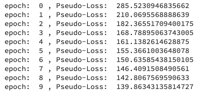
we can see that the pseudo-loss decreases steadily.
Once the model is trained we can generate samples using a Gibbs sampler that is built in the RBM class. After 10 epochs:
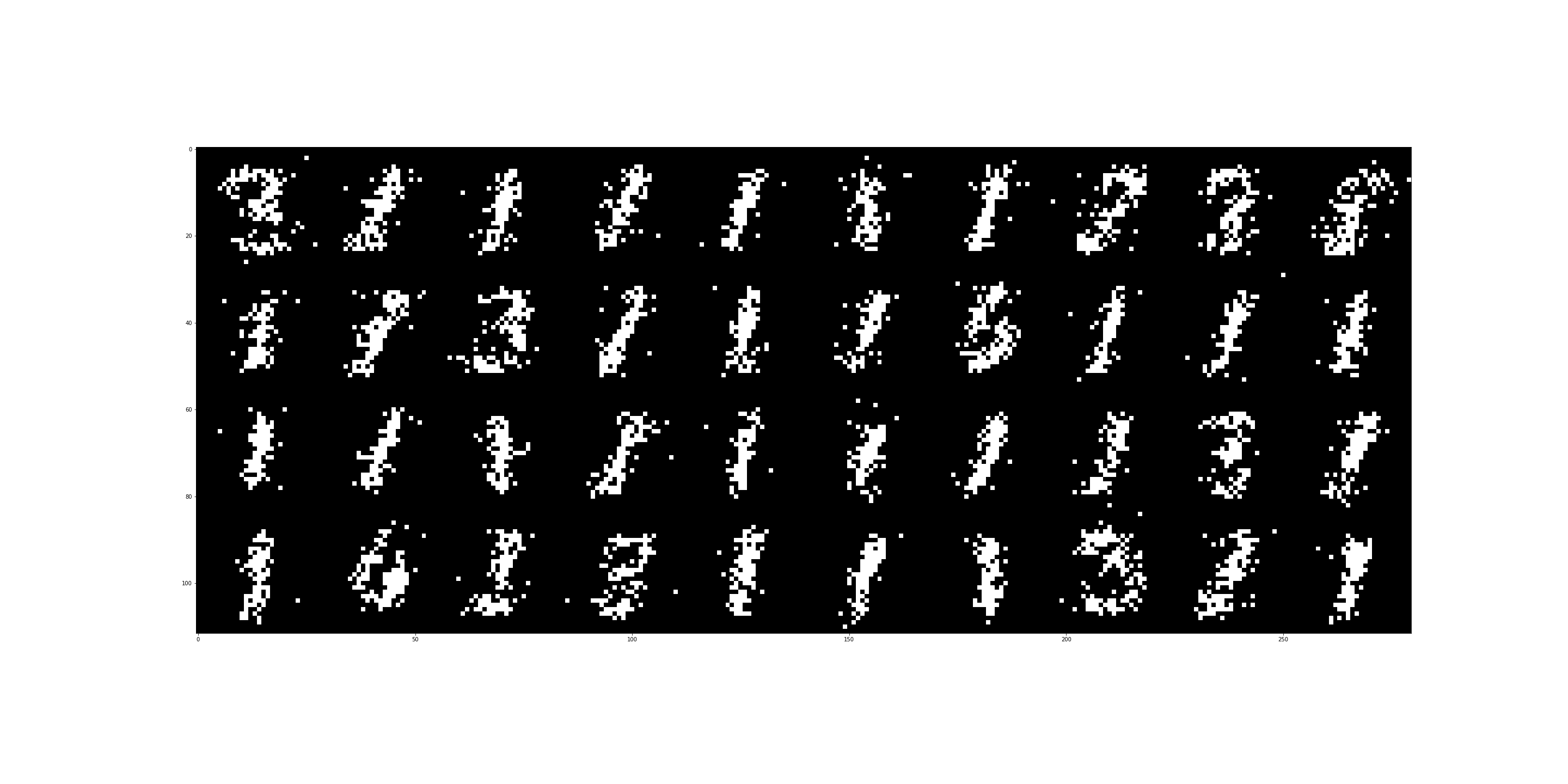
After 20 epochs:
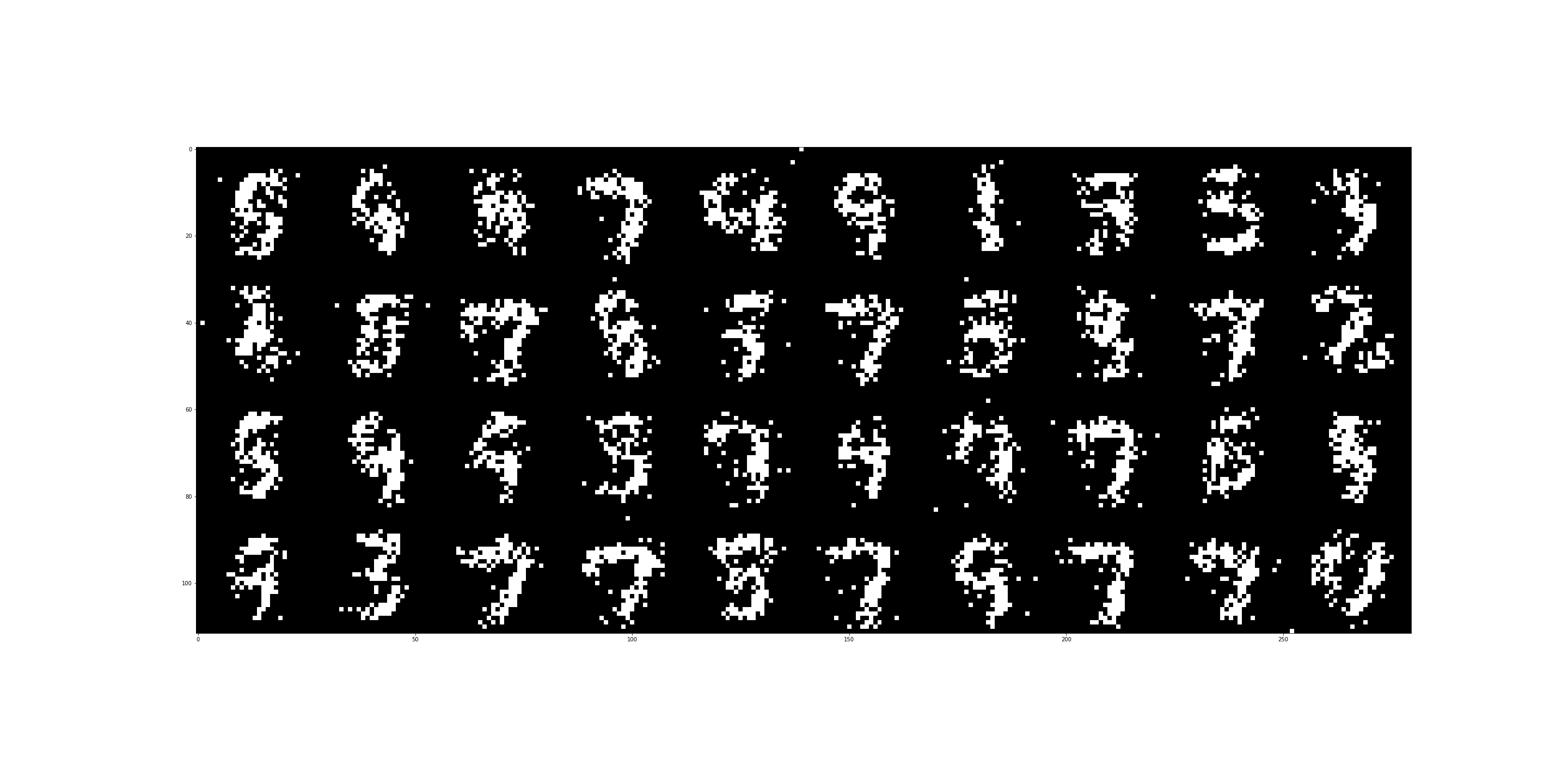
And finally after 40 epochs:
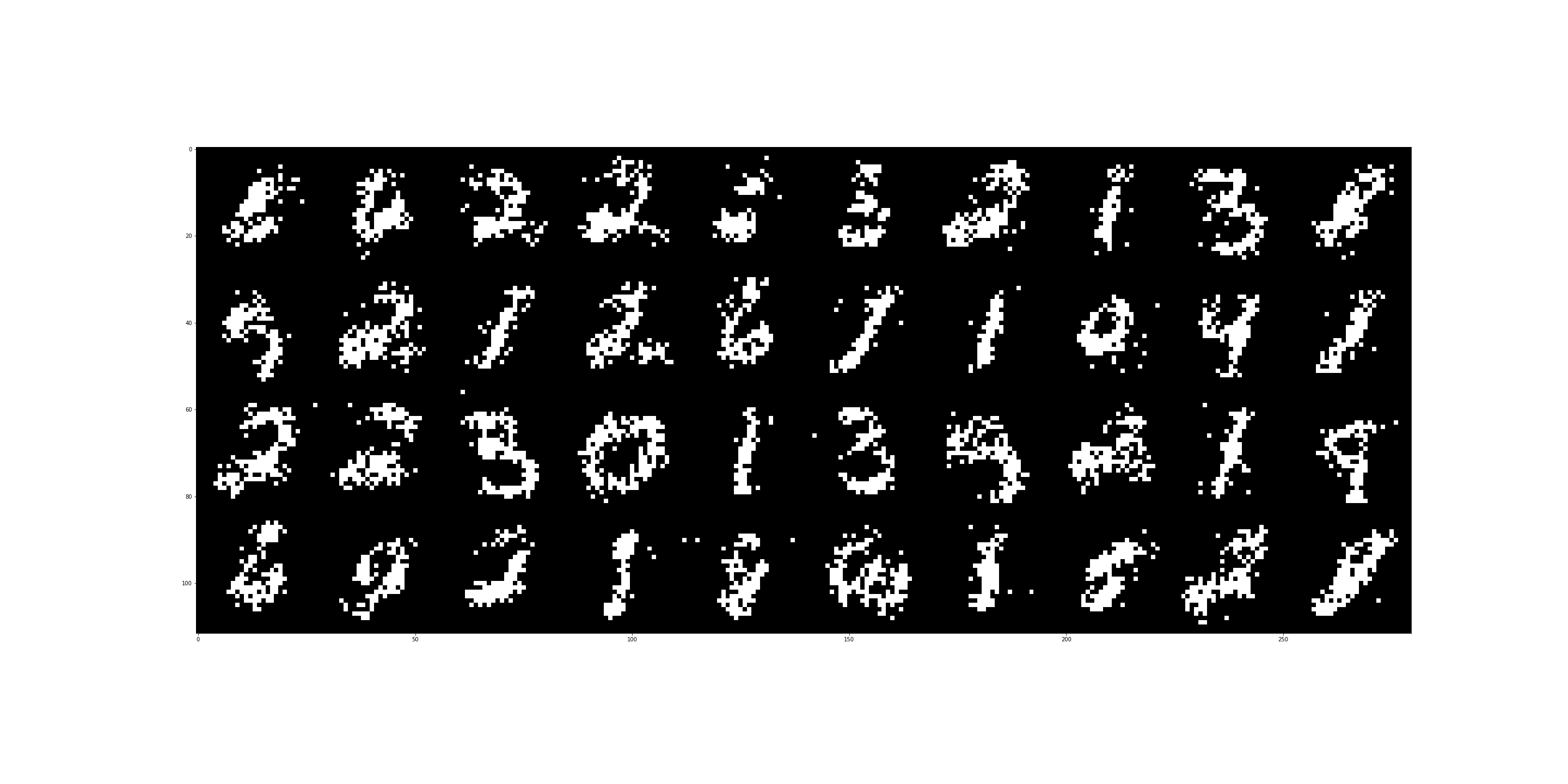
We see that with longer training the generated samples show more differentiation.
References
[1] A Practical Guide to Training Restricted Boltzmann Machines, G. Hinton, (2010)
[2] An Efficient Learning Procedure for Deep Boltzmann Machines, G. Hinton, R. Salakhutdinov (2012)
[3] Deep Learning, A. Courville, I. Goodfellow, Y. Bengio, (book)