Receiver Operating Curve
ROC curve
In a binary classification problem, the machine learning model calculates the probability of assigning label $y=1$ to the feature vector $x$
\[p(y=1|x)\]The optimal bayes predictor corresponds to labeling the data as
\[\hat{y}=1,\, \text{if }p(y=1|x)>p(y=0|x)\,\text{else }\hat{y}=0\]or equivalently $\hat{y}=1$ if $p(y=1|x)>0.5$. Recall that the optimal bayes predictor gives the best accuracy of all the predictors, provided that $p$ is the actual true probability. In some cases, the optimal bayes threshold $p>0.5$ is not the most useful. This can happen for example when the dataset is very unbalanced, meaning that the proportion of data-points with $y=1$ and $y=0$ is very different from 1. In this case, the accuracy is not most the appropriate metric. Note that the accuracy is defined as
\[\text{Accuracy}=\frac{ |y = \hat{y}| }{N}\]With $N_0$ and $N_1$ the number of data-points with labels $0,1$ respectively, we write
\[\begin{equation*}\begin{split}\text{Accuracy}& = \frac{ |y_0 = \hat{y}| + |y_1 = \hat{y}| }{N_0+N_1}=\frac{ N_0(|y_0 = \hat{y}|/N_0) + N_1(|y_1 = \hat{y}|/N_1) }{N_0+N_1}\\ &=r_0 \text{TNR}+r_1 \text{TPR}\end{split}\end{equation*}\]where $\text{TNR}$ is the true negative rate and $\text{TPR}$ is the true positive rate. The cofficients $r_1,r_0\equiv 1-r_1$ are the proportions of labels $1$ and $0$, respectively.
If we have a very unbalaced dataset, for example, with $r_1=1\%$ and $r_0=99\%$, then the predictor $\hat{y}=0$, that is, a constant, will achieve $99\%$ accuracy- the $\text{TPR}=0$ and $\text{TNR}=1$. This is, of course, a very misleading result because the predictor has no ability of distinguishing the classes.
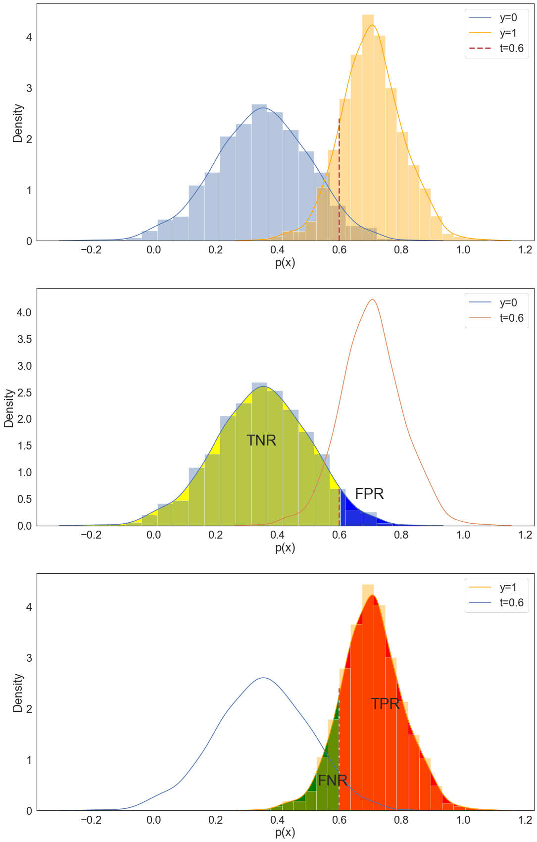
To circumvent this problem we need a metric that does not rely on the proportions $r_1,r_0$. The receiver operating curve, or ROC in short, is such a metric. We consider the distributions of the probability $p(y=1|x)$ separately for the data-points with labels $1,0$. See figure below

A perfect model is one for which the distributions do not overlap. Meaning that we can choose a threshold for $p(y=1|x)$ that achieves zero error, that is, $\text{TPR}=1$ and $\text{FPR}=0$. The idea of the ROC curve is to find the optimal threshold $t$ such that the predictor
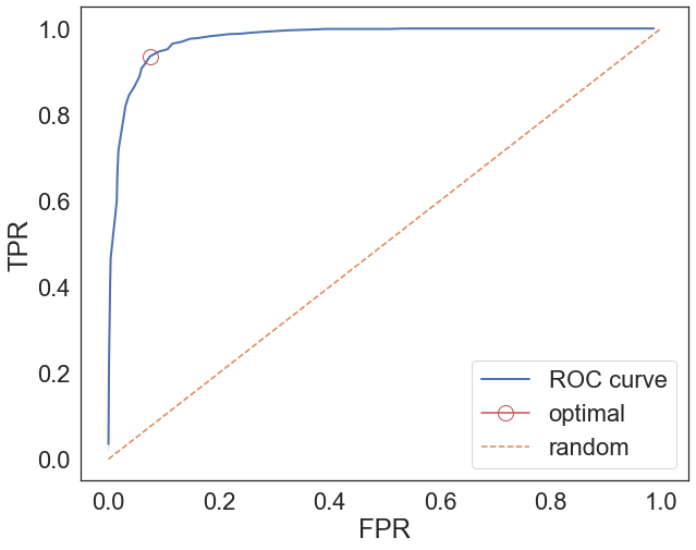
\[\hat{y}=1,\, \text{if }p(y=1|x)>t\,\text{else }\hat{y}=0\]guarantees the best generalization properties. To do this we explore a range of thresholds and calculate the corresponding $\text{TPR}(t)$ and $\text{FPR}(t)$ as a function of the threshold $t$.

The optimal threshold can be calculated as the point closest to the upper left corner.
Area Under the Curve: AUC
The area under the curve, or AUC, is an important metric. The model that achieves zero error has an $AUC=1$. By defintion we have
\[\text{AUC}=\int d\text{FPR}\,\text{TPR}\]The AUC is the probability that chosen two random samples with opposite labels $x_0$ and $x_1$, one has
\[p(y=1|x_1)>p(y=1|x_0)\]that is, a measure of discriminating the data-points in different classes. To see this, we need to calculate the probability
\[P(p(x_1)>p(x_0))\]Using a moving threshold $t$, this probability can be written as
\[P(p(x_1)>p(x_0))=\lim_{\Delta T\rightarrow 0}\sum_{t} P(p(x_1)>t)P(t\geq p(x_0)>t-\Delta t)\]and since
\[P(t\geq p(x_0)>t-\Delta t)=P(t\geq p(x_0))-P(t-\Delta t\geq p(x_0))=\frac{dP}{dt}\Delta t\]As $t$ increases, and so does the $\text{TNR}$. Therefore
\[\frac{dP}{dt}=\frac{d\text{TNR}}{dt}=-\frac{d\text{FPR}}{dt}\]So we conclude that
\[\begin{equation*}\begin{split} P(p(x_1)>p(x_0))&=-\int_0^1 dt \text{TPR}(t)\frac{d\text{FPR}}{dt}=-\int_{\text{FPR}(0)}^{\text{FPR}(1)} d\text{FPR}\,\text{TPR}\\ &=\int_{0}^{1} d\text{FPR}\,\text{TPR}\end{split}\end{equation*}\]One can distinguish essentialy three different types of ROC curves:

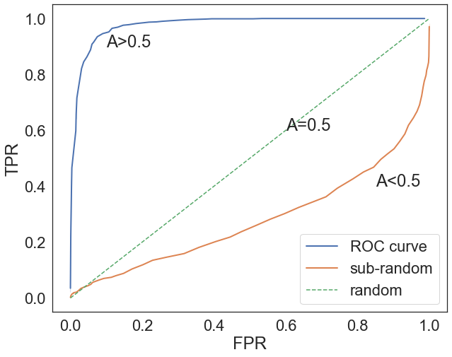
- A diagonal line: since it covers half of the area, it corresponds to a model with $P(p(x_1)>p(x_0))=0.5$, that is, a model that does as well as random choice.
- A curve above the diagonal: this means that $\text{AUC}>0.5$.
- A curve below the diagonal: this means that $\text{AUC}<0.5$. In this case, the model is doing worse than random chance. Not only it does not distinguish the labels, but it is mistakingly labeling the labels $y=1$ with $\hat{y}=0$ and vice-versa.
Python Implementation
class AUC:
    def __init__(self,y_true,y_score):
        ts=np.arange(0,1.02,0.01).reshape(1,-1)
        idx_0=(y_true==0)
        idx_1=(y_true==1)

        y_pred=(y_score.reshape(-1,1)>=ts).astype('int')
        self.fpr=y_pred[idx_0].mean(0)
        self.tpr=y_pred[idx_1].mean(0)

    def plot_roc(self):

        plt.plot(self.fpr,self.tpr)
        plt.show()

    def area(self):
        idx=np.argsort(self.fpr)
        x=self.fpr[idx]
        y=self.tpr[idx]
        A=0.5*(y[1:]+y[:-1])*(x[1:]-x[:-1])

        return A.sum()